Show code
pacman::p_load(sf, tmap, funModeling, maptools, spatstat, tidyverse, raster, sfdep)Discover the geographical distribution of functional and non-function water points in Osun State, Nigeria
Here, you will find a list with the data used, its type, format, and source it was extracted from.
| Type | Data | Format | Source |
|---|---|---|---|
| Geospatial | State GIS boundary data of Nigeria - Administration Level 1, 2 & 3 | .shp | OCHA data, extracted from the Humanitarian Data Exchange portal (data) |
| Geospatial | State GIS boundary data of Nigeria - Administration Level 2 | .shp | Data collected from geoboundaries.org |
| Aspatial | Water Point Data Exchange Plus | .csv | Data extracted from WPdx Global Data Repositories |
Note that the geoboundaries and OCHA data serve the same purpose. I decided to included both data set before choosing the most convenient one, based on a practical analysis of the variables included in the data sets.
For the purpose of our analysis, we will be using the following libraries:
sf
tmap
spatstat
raster
maptools
funModeling
tidyverse and readr, dplyr, ggplot2 & tidyr dependencies
pacman
To installl and load the packages, we will be using the function p_load() of the pacman package. This will ensure that all packages are installed and loaded properly.
pacman::p_load(sf, tmap, funModeling, maptools, spatstat, tidyverse, raster, sfdep)We use the read_csv() function from the readr package. This allows us to import the water point file into our R notebook. We will store the data set under the variable wp_nga.
wp_nga = read_csv("data/aspatial/Water_Point_Data_Exchange_-_Plus__WPdx__.csv", show_col_types = FALSE)Before diving into Data Wrangling, the first step is to get an understanding of the data and its attributes. By using the function glimpse() of the dplyr package, we will be able to view the attributes of this data set and data type of each field.
glimpse(wp_nga)Rows: 406,566
Columns: 70
$ row_id <dbl> 651816, 584864, 509399, 21983, 660321, 6…
$ `#source` <chr> "Water For People", "Global Environment …
$ `#lat_deg` <dbl> -15.726464200, 6.723120000, 8.001933333,…
$ `#lon_deg` <dbl> 35.05067, -1.58151, -11.28760, -10.12595…
$ `#report_date` <chr> "06/11/2018 12:00:00 AM", "10/25/2017 12…
$ `#status_id` <chr> "Yes", "Yes", "Yes", "Yes", "Yes", "Yes"…
$ `#water_source_clean` <chr> NA, NA, NA, NA, "Piped Water", "Piped Wa…
$ `#water_source_category` <chr> NA, NA, NA, NA, "Piped Water", "Piped Wa…
$ `#water_tech_clean` <chr> "Kiosk", "Tapstand", "Tapstand", "Tapsta…
$ `#water_tech_category` <chr> "Tapstand", "Tapstand", "Tapstand", "Tap…
$ `#facility_type` <chr> "Improved", "Improved", "Improved", "Imp…
$ `#clean_country_name` <chr> "Malawi", "Ghana", "Sierra Leone", "Libe…
$ `#clean_adm1` <chr> "Blantyre", "Ashanti", "Eastern", "Lofa"…
$ `#clean_adm2` <chr> "Blantyre City", "Asokore Mampong Munici…
$ `#clean_adm3` <chr> "n.a. (2465)", NA, "Kando Leppeama", "Lu…
$ `#clean_adm4` <chr> NA, NA, NA, NA, "Kamwenge Town Council",…
$ `#install_year` <dbl> NA, 2017, NA, NA, NA, NA, NA, NA, NA, NA…
$ `#installer` <chr> NA, NA, "Water Aid", NA, NA, NA, NA, NA,…
$ `#rehab_year` <lgl> NA, NA, NA, NA, NA, NA, NA, NA, NA, NA, …
$ `#rehabilitator` <lgl> NA, NA, NA, NA, NA, NA, NA, NA, NA, NA, …
$ `#management_clean` <chr> NA, NA, NA, "School Management", NA, NA,…
$ `#status_clean` <chr> NA, NA, "Functional", NA, NA, NA, NA, NA…
$ `#pay` <chr> NA, NA, NA, NA, NA, NA, NA, NA, NA, NA, …
$ `#fecal_coliform_presence` <chr> NA, NA, NA, NA, "Present", "Present", "P…
$ `#fecal_coliform_value` <dbl> NA, 0, NA, NA, NA, NA, NA, NA, NA, NA, N…
$ `#subjective_quality` <chr> NA, NA, NA, NA, NA, NA, NA, NA, NA, NA, …
$ `#activity_id` <chr> NA, NA, NA, NA, NA, NA, NA, NA, NA, NA, …
$ `#scheme_id` <chr> NA, NA, NA, NA, NA, NA, NA, NA, NA, NA, …
$ `#wpdx_id` <chr> "5GPQ73F2+C77", "6CRWPCF9+69X", "6CWC2P2…
$ `#notes` <chr> NA, NA, "Poor…Jenneh…Kandu Leppiema……", …
$ `#orig_lnk` <chr> NA, NA, NA, "https://wash-liberia.org/ra…
$ `#photo_lnk` <chr> NA, NA, NA, NA, NA, NA, NA, NA, NA, NA, …
$ `#country_id` <chr> "MW", "GH", "SL", "LR", "UG", "UG", "UG"…
$ `#data_lnk` <chr> "https://catalog.waterpointdata.org/data…
$ `#distance_to_primary_road` <dbl> 7034.8250, 3677.9101, 17540.3622, 21602.…
$ `#distance_to_secondary_road` <dbl> 3431.81039, 3944.70081, 4052.93329, 3703…
$ `#distance_to_tertiary_road` <dbl> 421.90674, 690.13048, 104.43156, 14456.7…
$ `#distance_to_city` <dbl> 8321.854, 5362.011, 17003.136, 52727.389…
$ `#distance_to_town` <dbl> 22044.5149, 7550.3392, 15474.4428, 31606…
$ water_point_history <chr> "{\"2018-06-11\": {\"source\": \"Water F…
$ rehab_priority <dbl> NA, NA, NA, NA, NA, NA, NA, NA, NA, NA, …
$ water_point_population <dbl> NA, NA, NA, NA, NA, NA, NA, NA, NA, NA, …
$ local_population_1km <dbl> NA, NA, NA, NA, NA, NA, NA, NA, NA, NA, …
$ crucialness_score <dbl> NA, NA, NA, NA, NA, NA, NA, NA, NA, NA, …
$ pressure_score <dbl> NA, NA, NA, NA, NA, NA, NA, NA, NA, NA, …
$ usage_capacity <dbl> 250, 250, 250, 250, 250, 250, 250, 250, …
$ is_urban <lgl> TRUE, TRUE, FALSE, FALSE, FALSE, FALSE, …
$ days_since_report <dbl> 1562, 1791, 4281, 2482, 1286, 1281, 1660…
$ staleness_score <dbl> 61.11805, 56.86178, 25.93887, 45.73258, …
$ latest_record <lgl> TRUE, TRUE, TRUE, TRUE, TRUE, TRUE, TRUE…
$ location_id <dbl> 355848, 349148, 98255, 285679, 362508, 3…
$ cluster_size <dbl> 1, 1, 1, 1, 1, 1, 1, 2, 1, 1, 1, 1, 1, 1…
$ `#clean_country_id` <chr> "MWI", "GHA", "SLE", "LBR", "UGA", "UGA"…
$ `#country_name` <chr> "Malawi", "Ghana", "Sierra Leone", "Libe…
$ `#water_source` <chr> NA, NA, "Gravity stand-post", "Public st…
$ `#water_tech` <chr> "Communal water kiosk", "Standpost", NA,…
$ `#status` <chr> "1", NA, "Functional", NA, "1", "0", "1"…
$ `#adm2` <chr> "Kameza", NA, "Kenema", NA, "Kibale", "K…
$ `#adm3` <chr> NA, NA, NA, NA, "Kamwenge T/Council", "B…
$ `#management` <chr> NA, NA, NA, "Institutional Management - …
$ `#adm1` <chr> "Blantyre", NA, "Eastern", "Lofa", "Kamw…
$ `New Georeferenced Column` <chr> "POINT (35.0506729 -15.7264642)", "POINT…
$ lat_deg_original <dbl> NA, NA, NA, NA, NA, NA, NA, NA, NA, NA, …
$ lat_lon_deg <chr> "(-15.7264642°, 35.0506729°)", "(6.72312…
$ lon_deg_original <dbl> NA, NA, NA, NA, NA, NA, NA, NA, NA, NA, …
$ public_data_source <chr> "https://catalog.waterpointdata.org/data…
$ converted <chr> NA, NA, "#install_year, #notes", "#statu…
$ count <dbl> 1, 1, 1, 1, 1, 1, 1, 1, 1, 1, 1, 1, 1, 1…
$ created_timestamp <chr> "02/18/2022 05:36:33 AM", "07/29/2020 07…
$ updated_timestamp <chr> "02/18/2022 05:36:33 AM", "07/29/2020 07…The output reveals that we have a tible data frame – wp_nga – composed of 406,566 data points and 70 columns. It is now time to take a few seconds to browse through the data to get a proper look at the different attributes in the data set.
Since our goal is to observe data only from the Osun state in Nigeria, we should take a look at the attributes that will allow us to filter the data set. It seems like the columns: clean_country_name & clean_adm1 contain the information about the country and state of the water points.
Using the filter() function, we will be to select on data points from the Osun state in Nigeria.
wp_nga = wp_nga %>%
  filter(`#clean_country_name` == "Nigeria" & `#clean_adm1` == "Osun")
To check if there are no mistake, we can use the function unique() to help us view all the unique strings in the columns clean_country_name & clean_adm1
unique(wp_nga$`#clean_adm1`); unique(wp_nga$`#clean_country_name`)[1] "Osun"[1] "Nigeria"We obtained the desired output, we are only left with data points located in Osun state, Nigeria
Using the st_as_sfc() function of the sf package, we convert the wkt field – `New Georeferenced Column` –into a sfc field.
wp_nga$Geometry = st_as_sfc(wp_nga$`New Georeferenced Column`)
wp_nga
# A tibble: 5,557 × 71
row_id `#source` #lat_…¹ #lon_…² #repo…³ #stat…⁴ #wate…⁵ #wate…⁶ #wate…⁷
<dbl> <chr> <dbl> <dbl> <chr> <chr> <chr> <chr> <chr>
1 429123 GRID3 8.02 5.06 08/29/… Unknown <NA> <NA> Tapsta…
2 70566 Federal Minis… 7.32 4.79 05/11/… No Protec… Well Mechan…
3 70578 Federal Minis… 7.76 4.56 05/11/… No Boreho… Well Mechan…
4 66401 Federal Minis… 8.03 4.64 04/30/… No Boreho… Well Mechan…
5 422190 GRID3 7.87 4.88 08/29/… Unknown <NA> <NA> Tapsta…
6 422064 GRID3 7.7 4.89 08/29/… Unknown <NA> <NA> Tapsta…
7 65607 Federal Minis… 7.89 4.71 05/12/… No Boreho… Well Mechan…
8 68989 Federal Minis… 7.51 4.27 05/07/… No Boreho… Well <NA>
9 67708 Federal Minis… 7.48 4.35 04/29/… Yes Boreho… Well Mechan…
10 66419 Federal Minis… 7.63 4.50 05/08/… Yes Boreho… Well Hand P…
# … with 5,547 more rows, 62 more variables: `#water_tech_category` <chr>,
# `#facility_type` <chr>, `#clean_country_name` <chr>, `#clean_adm1` <chr>,
# `#clean_adm2` <chr>, `#clean_adm3` <chr>, `#clean_adm4` <chr>,
# `#install_year` <dbl>, `#installer` <chr>, `#rehab_year` <lgl>,
# `#rehabilitator` <lgl>, `#management_clean` <chr>, `#status_clean` <chr>,
# `#pay` <chr>, `#fecal_coliform_presence` <chr>,
# `#fecal_coliform_value` <dbl>, `#subjective_quality` <chr>, …Now, we can convert the tibble data frame into a sf object using the st_sf() function. We shall also specify the georeferencing system (crs code). Here, it seems like the data is referenced in WGS84.
wp_sf <- wp_nga %>%
  st_sf(crs=4326)
wp_sf
Simple feature collection with 5557 features and 70 fields
Geometry type: POINT
Dimension: XY
Bounding box: xmin: 4.032004 ymin: 7.060309 xmax: 5.06 ymax: 8.061898
Geodetic CRS: WGS 84
# A tibble: 5,557 × 71
row_id `#source` #lat_…¹ #lon_…² #repo…³ #stat…⁴ #wate…⁵ #wate…⁶ #wate…⁷
* <dbl> <chr> <dbl> <dbl> <chr> <chr> <chr> <chr> <chr>
1 429123 GRID3 8.02 5.06 08/29/… Unknown <NA> <NA> Tapsta…
2 70566 Federal Minis… 7.32 4.79 05/11/… No Protec… Well Mechan…
3 70578 Federal Minis… 7.76 4.56 05/11/… No Boreho… Well Mechan…
4 66401 Federal Minis… 8.03 4.64 04/30/… No Boreho… Well Mechan…
5 422190 GRID3 7.87 4.88 08/29/… Unknown <NA> <NA> Tapsta…
6 422064 GRID3 7.7 4.89 08/29/… Unknown <NA> <NA> Tapsta…
7 65607 Federal Minis… 7.89 4.71 05/12/… No Boreho… Well Mechan…
8 68989 Federal Minis… 7.51 4.27 05/07/… No Boreho… Well <NA>
9 67708 Federal Minis… 7.48 4.35 04/29/… Yes Boreho… Well Mechan…
10 66419 Federal Minis… 7.63 4.50 05/08/… Yes Boreho… Well Hand P…
# … with 5,547 more rows, 62 more variables: `#water_tech_category` <chr>,
# `#facility_type` <chr>, `#clean_country_name` <chr>, `#clean_adm1` <chr>,
# `#clean_adm2` <chr>, `#clean_adm3` <chr>, `#clean_adm4` <chr>,
# `#install_year` <dbl>, `#installer` <chr>, `#rehab_year` <lgl>,
# `#rehabilitator` <lgl>, `#management_clean` <chr>, `#status_clean` <chr>,
# `#pay` <chr>, `#fecal_coliform_presence` <chr>,
# `#fecal_coliform_value` <dbl>, `#subjective_quality` <chr>, …Using the function st_transform(), we transform the sf coordinates of our data points into the Nigerian projected coordinate system.
Note that there are three Projected Coordinate Systems of Nigeria, they are: EPSG: 26391, 26392, and 26303. For the purpose of our analysis, we will choose EPSG: 26391.
wp_sf <- wp_sf %>%
st_transform(crs = 26391)We use the function st_read() from sf package to import our geospatial data. Here, we import the NGA data set, which is stored in our data folder as a shp file. Since our analysis is focused on the Osun State (Nigeria), we will use the filter() function to select the data corresponding to the Administration Level 1 of Osun State.
nga = st_read(dsn = "data/geospatial",
                   layer = "nga_admbnda_adm2") %>%
  filter(ADM1_EN == "Osun")
Reading layer `nga_admbnda_adm2' from data source
`C:\p-haas\IS415\Take-home_Ex\Take-home_Ex01\data\geospatial'
using driver `ESRI Shapefile'
Simple feature collection with 774 features and 16 fields
Geometry type: MULTIPOLYGON
Dimension: XY
Bounding box: xmin: 2.668534 ymin: 4.273007 xmax: 14.67882 ymax: 13.89442
Geodetic CRS: WGS 84Before proceeding to the next steps, I would like to retrieve the CRS code from the sf object to perform a quick check that the CRS and code match. To do so, we use the st_crs() function which helps us do that.
st_crs(nga)Coordinate Reference System:
User input: WGS 84
wkt:
GEOGCRS["WGS 84",
DATUM["World Geodetic System 1984",
ELLIPSOID["WGS 84",6378137,298.257223563,
LENGTHUNIT["metre",1]]],
PRIMEM["Greenwich",0,
ANGLEUNIT["degree",0.0174532925199433]],
CS[ellipsoidal,2],
AXIS["latitude",north,
ORDER[1],
ANGLEUNIT["degree",0.0174532925199433]],
AXIS["longitude",east,
ORDER[2],
ANGLEUNIT["degree",0.0174532925199433]],
ID["EPSG",4326]]The CRS and id match, therefore we can move on to the next step and transform the data into the Nigerian projected coordinate system.
As explained before, using st_transform(), we convert the sf coordinates into the Nigerian projected coordinate system.
nga <- nga %>%
  st_transform(crs = 26391)
nga
Simple feature collection with 30 features and 16 fields
Geometry type: MULTIPOLYGON
Dimension: XY
Bounding box: xmin: 178398.7 ymin: 329463.4 xmax: 292278.9 ymax: 452734.9
Projected CRS: Minna / Nigeria West Belt
First 10 features:
Shape_Leng Shape_Area ADM2_EN ADM2_PCODE ADM2_REF ADM2ALT1EN
1 1.7951405 0.062436080 Aiyedade NG030001 Aiyedade <NA>
2 0.7101503 0.024818478 Aiyedire NG030002 Aiyedire <NA>
3 0.9199564 0.038002894 Atakumosa East NG030003 Atakumosa East <NA>
4 0.8502782 0.030445804 Atakumosa West NG030004 Atakumosa West <NA>
5 0.5212768 0.012213340 Boluwaduro NG030005 Boluwaduro <NA>
6 0.6088930 0.011827501 Boripe NG030006 Boripe <NA>
7 0.4714403 0.008343638 Ede North NG030007 Ede North <NA>
8 0.5660235 0.017623677 Ede South NG030008 Ede South <NA>
9 0.8273123 0.022026327 Egbedore NG030009 Egbedore <NA>
10 1.1304849 0.029791275 Ejigbo NG030010 Ejigbo <NA>
ADM2ALT2EN ADM1_EN ADM1_PCODE ADM0_EN ADM0_PCODE date validOn
1 <NA> Osun NG030 Nigeria NG 2016-11-29 2019-04-17
2 <NA> Osun NG030 Nigeria NG 2016-11-29 2019-04-17
3 <NA> Osun NG030 Nigeria NG 2016-11-29 2019-04-17
4 <NA> Osun NG030 Nigeria NG 2016-11-29 2019-04-17
5 <NA> Osun NG030 Nigeria NG 2016-11-29 2019-04-17
6 <NA> Osun NG030 Nigeria NG 2016-11-29 2019-04-17
7 <NA> Osun NG030 Nigeria NG 2016-11-29 2019-04-17
8 <NA> Osun NG030 Nigeria NG 2016-11-29 2019-04-17
9 <NA> Osun NG030 Nigeria NG 2016-11-29 2019-04-17
10 <NA> Osun NG030 Nigeria NG 2016-11-29 2019-04-17
validTo SD_EN SD_PCODE geometry
1 <NA> Osun West NG03003 MULTIPOLYGON (((215920.8 33...
2 <NA> Osun West NG03003 MULTIPOLYGON (((214352.3 40...
3 <NA> Osun East NG03002 MULTIPOLYGON (((267717.8 37...
4 <NA> Osun East NG03002 MULTIPOLYGON (((250576.1 40...
5 <NA> Osun Central NG03001 MULTIPOLYGON (((267547.9 42...
6 <NA> Osun Central NG03001 MULTIPOLYGON (((256469.1 43...
7 <NA> Osun West NG03003 MULTIPOLYGON (((238094.5 40...
8 <NA> Osun West NG03003 MULTIPOLYGON (((238094.5 40...
9 <NA> Osun West NG03003 MULTIPOLYGON (((222300.9 42...
10 <NA> Osun West NG03003 MULTIPOLYGON (((216011.1 42...The projected CRS now corresponds to the Nigerian one, we will be able to perform data wrangling from now on.
In this section, we will follow the same steps as the NGA data set but for the geoBoundaries data this time, however, since we will choose the NGA data over the latter, we can refrain from performing the next steps. Yet, I include the code if one chooses to work with the geoBoundaries data set.
geoNGA = st_read(dsn = "data/geospatial",
layer = "geoBoundaries-NGA-ADM2")st_crs(geoNGA)geoNGA <- geoNGA %>%
st_transform(crs = 26391)
geoNGATo simplify our work, we shall reduce our data set and use only necessary attributes. Using the select() function, we will choose fields 3, 4, 8, and 9. By doing so, we exclude redundant fields.
nga <- nga %>%
  dplyr::select(c(3:4, 8:9))
Note that the Geometry field remains in our sf data frame.
Checking for duplicates is an essential part of data cleaning. Here, we shall check if any … have the same name within the Osun State.
nga$ADM2_EN[duplicated(nga$ADM2_EN)==TRUE]character(0)There are no duplicates in the data set. We shall then move on to the data wrangling of the water points.
Given the nature of our work which focuses on analyzing the distribution of functional and non-functional water points throughout the Osun State in Nigeria, we should explore the attribute that stores such information.
Looking back at the previous work done, it seems that the field #status_clean indicates the nature of the water point. By using the freq() function from the funModeling package, we display the information about the water points on a bar plot.
funModeling::freq(data = wp_sf,
     input = '#status_clean')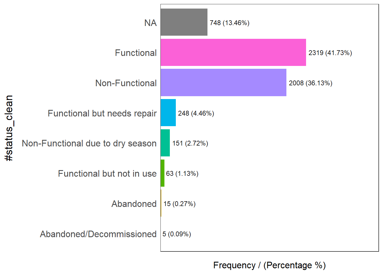
                     #status_clean frequency percentage cumulative_perc
1                       Functional      2319      41.73           41.73
2                   Non-Functional      2008      36.13           77.86
3                             <NA>       748      13.46           91.32
4      Functional but needs repair       248       4.46           95.78
5 Non-Functional due to dry season       151       2.72           98.50
6        Functional but not in use        63       1.13           99.63
7                        Abandoned        15       0.27           99.90
8         Abandoned/Decommissioned         5       0.09          100.00
Looking at the above bar plot, we learn that:
15% of observations are not classified, we should treat that issue next;
the functional water points are classified into 3 categories, namely “Functional”, “Functional but needs repair”, and “Functional but in use”;
the non-functional water points are classified into 4 categories, namely “Non-Functional”, “Non-Functional due to dry season”, “Abandoned”, and “Abandoned/Decommissioned”;
Before extracting the water point data, we will simplify our work by creating an alternate data frame using the rename(), select(), and mutate() functions.
We use rename() to rename the ‘#status_clean’ field to status_clean, it will make data handling easier;
We use select() of the dplyr package to include the status_clean attribute in the output sf data frame;
We use replace_na() to change all NA values from the status_clean column into unknown.
wp_sf_nga <- wp_sf %>%
  rename(status_clean = '#status_clean') %>%
  dplyr::select(status_clean) %>%
  mutate(status_clean = replace_na(
    status_clean, "unknown"))
head(wp_sf_nga)
Simple feature collection with 6 features and 1 field
Geometry type: POINT
Dimension: XY
Bounding box: xmin: 237881.5 ymin: 366733.1 xmax: 292542.7 ymax: 445609.1
Projected CRS: Minna / Nigeria West Belt
# A tibble: 6 × 2
status_clean Geometry
<chr> <POINT [m]>
1 unknown (292542.7 444411.7)
2 Abandoned/Decommissioned (262341.4 366733.1)
3 Abandoned/Decommissioned (237881.5 415561.5)
4 Abandoned/Decommissioned (245966.3 445609.1)
5 unknown (272719.3 427803.4)
6 unknown (273839.2 409007.6)In order to perform tests on the different water point categories, we should extract the water point data according to their status. We will use the function filter() to do so, and shall include all relevant categories to functional and non-functional water points as mentioned earlier.
wp_sf_functional <- wp_sf_nga %>%
  filter(status_clean %in%
           c("Functional",
             "Functional but not in use",
"Functional but needs repair"))funModeling::freq(data = wp_sf_functional,
input = 'status_clean')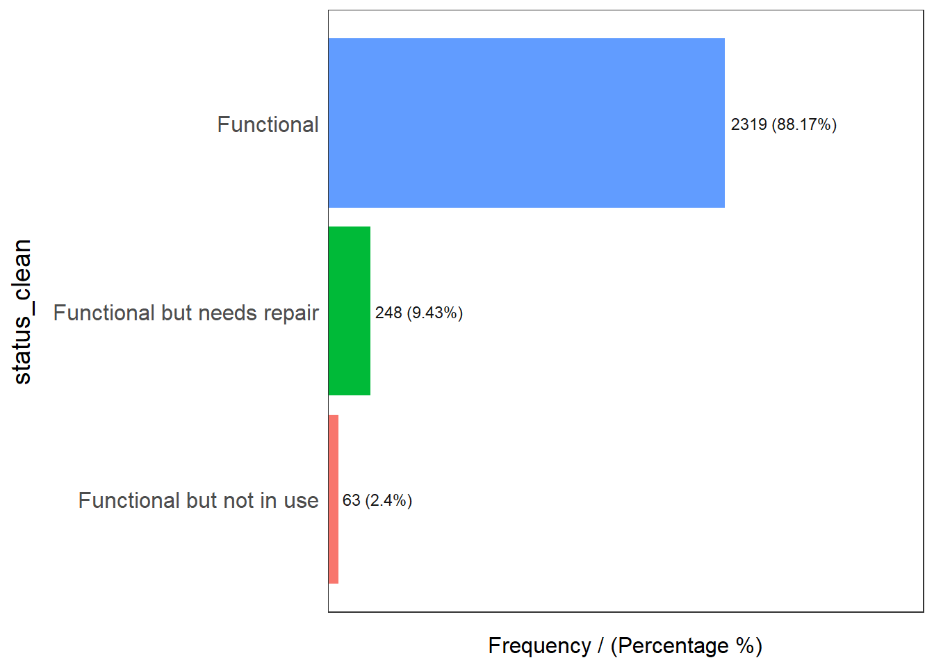
                 status_clean frequency percentage cumulative_perc
1                  Functional      2319      88.17           88.17
2 Functional but needs repair       248       9.43           97.60
3   Functional but not in use        63       2.40          100.00
wp_sf_nonfunctional <- wp_sf_nga %>%
filter(status_clean %in%
c("Abandoned/Decommissioned",
"Abandoned",
"Non-Functional due to dry season",
"Non-Functional"))funModeling::freq(data = wp_sf_nonfunctional,
input = 'status_clean')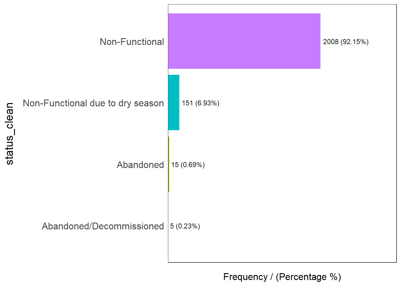
                      status_clean frequency percentage cumulative_perc
1                   Non-Functional      2008      92.15           92.15
2 Non-Functional due to dry season       151       6.93           99.08
3                        Abandoned        15       0.69           99.77
4 Abandoned/Decommissioned 5 0.23 100.00nga_wp <- nga %>%
mutate(`total_wp` = lengths(
st_intersects(nga, wp_sf_nga))) %>%
mutate(`wp_functional` = lengths(
st_intersects(nga, wp_sf_functional))) %>%
mutate(`wp_nonfunctional` = lengths(
st_intersects(nga, wp_sf_nonfunctional)))ggplot(data = nga_wp,
aes(x = wp_functional)) +
geom_histogram(bins=20,
color="black",
fill="light blue") +
geom_vline(aes(xintercept=mean(
wp_functional, na.rm=T)),
color="red",
linetype="dashed",
size=0.8) +
ggtitle("Distribution of Functional water points by LGA") +
xlab("No. of water points") +
ylab("No. of\nLGAs") +
theme(axis.title.y=element_text(angle = 0))
ggplot(data = nga_wp,
       aes(x = wp_functional)) +
  geom_histogram(bins=20,
                 color="black",
                 fill="light blue") +
  geom_vline(aes(xintercept=mean(
    wp_functional, na.rm=T)),
             color="red",
             linetype="dashed",
             size=0.8) +
  ggtitle("Distribution of Functional water points by LGA") +
  xlab("No. of water points") +
  ylab("No. of\nLGAs") +
  theme(axis.title.y=element_text(angle = 0))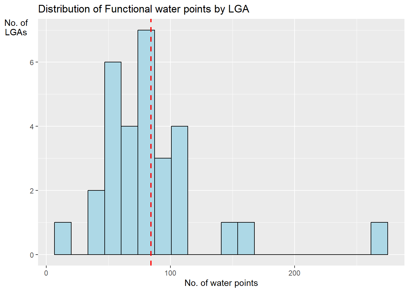
In order to perform first-order spatial point pattern analysis and plot kernel density estimation maps, a few necessary steps remain. Indeed, spatstat package requires us to use analytical data in ppp object form. We call that geospatial data wrangling. In the following parts, we will convert our sf data frames into ppp and owin objects.
Note that we will be working with the three following data frames:
wp_sf_functional, being the sf data frame that stores the geometry of functional water points;
wp_sf_nonfunctional, being the sf data frame that stores the geometry of non-functional water points;
nga, being the sf data frame that stores the geometry of level 2 administrative boundaries in Nigeria;
The first step to converting an sf data frame to a ppp class object is to use the as_Spatial() function of the sf package. It converts the geospatial data from sf data frame to sp’s Spatial* class.
Below, we perform this transformation on the three data frames.
wp_functional = as_Spatial(wp_sf_functional)
wp_functional
class : SpatialPointsDataFrame
features : 2630
extent : 179198.9, 291989.5, 341443.2, 449013.7 (xmin, xmax, ymin, ymax)
crs : +proj=tmerc +lat_0=4 +lon_0=4.5 +k=0.99975 +x_0=230738.26 +y_0=0 +a=6378249.145 +rf=293.465 +towgs84=-92,-93,122,0,0,0,0 +units=m +no_defs
variables : 1
names : status_clean
min values : Functional
max values : Functional but not in use Note that wp_functional is a Spatial Points data frame.
wp_nonfunctional = as_Spatial(wp_sf_nonfunctional)
wp_nonfunctional
class : SpatialPointsDataFrame
features : 2179
extent : 182490.7, 291855.5, 338261.8, 448933.5 (xmin, xmax, ymin, ymax)
crs : +proj=tmerc +lat_0=4 +lon_0=4.5 +k=0.99975 +x_0=230738.26 +y_0=0 +a=6378249.145 +rf=293.465 +towgs84=-92,-93,122,0,0,0,0 +units=m +no_defs
variables : 1
names : status_clean
min values : Abandoned
max values : Non-Functional due to dry season Note that wp_nonfunctional is a Spatial Points data frame.
nga_spat = as_Spatial(nga)
nga_spat
class : SpatialPolygonsDataFrame
features : 30
extent : 178398.7, 292278.9, 329463.4, 452734.9 (xmin, xmax, ymin, ymax)
crs : +proj=tmerc +lat_0=4 +lon_0=4.5 +k=0.99975 +x_0=230738.26 +y_0=0 +a=6378249.145 +rf=293.465 +towgs84=-92,-93,122,0,0,0,0 +units=m +no_defs
variables : 4
names : ADM2_EN, ADM2_PCODE, ADM1_EN, ADM1_PCODE
min values : Aiyedade, NG030001, Osun, NG030
max values : Osogbo, NG030030, Osun, NG030 Note that nga_spat is a Spatial Polygons data frame.
Since we are looking to convert the data frames to ppp objects and there are no direct methods to convert Spatial* classes into ppp objects, we shall find an alternative way. We need to convert the Spatial* classes into sp objects first. To do so, we use the as() function to coerce our Spatial* objects to their respective sp classes (e.g., ‘SpatialPoints’ and ‘SpatialPolygons’). We shall perform this transformation on our three data sets.
wp_functional_sp <- as(wp_functional, "SpatialPoints")
wp_functional_sp
class : SpatialPoints
features : 2630
extent : 179198.9, 291989.5, 341443.2, 449013.7 (xmin, xmax, ymin, ymax)
crs : +proj=tmerc +lat_0=4 +lon_0=4.5 +k=0.99975 +x_0=230738.26 +y_0=0 +a=6378249.145 +rf=293.465 +towgs84=-92,-93,122,0,0,0,0 +units=m +no_defs wp_nonfunctional_sp <- as(wp_nonfunctional, "SpatialPoints")
wp_nonfunctional_spclass : SpatialPoints
features : 2179
extent : 182490.7, 291855.5, 338261.8, 448933.5 (xmin, xmax, ymin, ymax)
crs : +proj=tmerc +lat_0=4 +lon_0=4.5 +k=0.99975 +x_0=230738.26 +y_0=0 +a=6378249.145 +rf=293.465 +towgs84=-92,-93,122,0,0,0,0 +units=m +no_defs nga_sp <- as(nga_spat, "SpatialPolygons")
nga_spclass : SpatialPolygons
features : 30
extent : 178398.7, 292278.9, 329463.4, 452734.9 (xmin, xmax, ymin, ymax)
crs : +proj=tmerc +lat_0=4 +lon_0=4.5 +k=0.99975 +x_0=230738.26 +y_0=0 +a=6378249.145 +rf=293.465 +towgs84=-92,-93,122,0,0,0,0 +units=m +no_defs wp_functional_ppp <- as(wp_functional_sp, "ppp")
wp_functional_pppPlanar point pattern: 2630 points
window: rectangle = [179198.89, 291989.51] x [341443.2, 449013.7] unitsplot(wp_functional_ppp)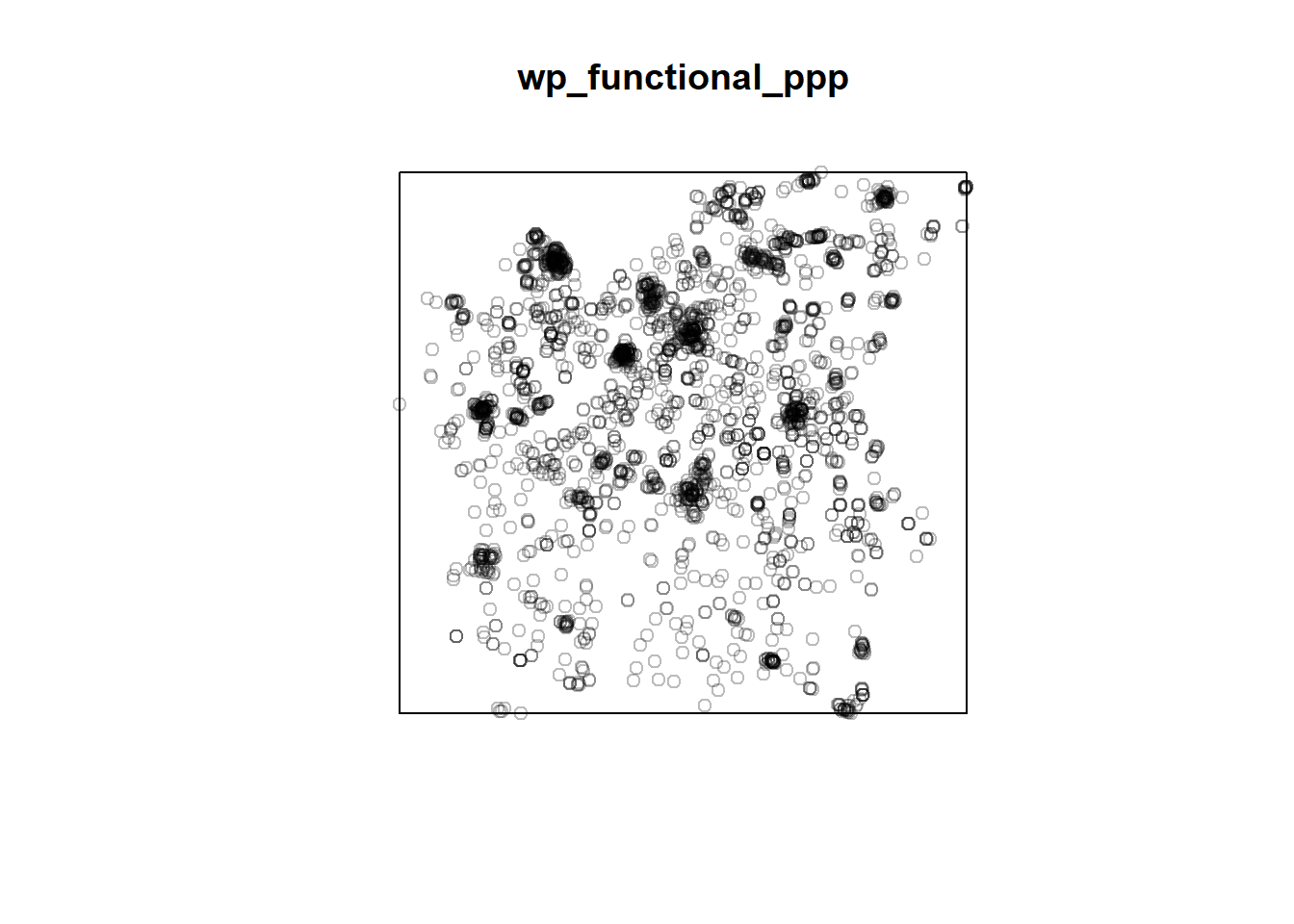
summary(wp_functional_ppp)Planar point pattern: 2630 points
Average intensity 2.167651e-07 points per square unit
Coordinates are given to 2 decimal places
i.e. rounded to the nearest multiple of 0.01 units
Window: rectangle = [179198.89, 291989.51] x [341443.2, 449013.7] units
(112800 x 107600 units)
Window area = 12132900000 square unitswp_nonfunctional_ppp <- as(wp_nonfunctional_sp, "ppp")
wp_nonfunctional_pppPlanar point pattern: 2179 points
window: rectangle = [182490.74, 291855.52] x [338261.8, 448933.5] unitsplot(wp_nonfunctional_sp)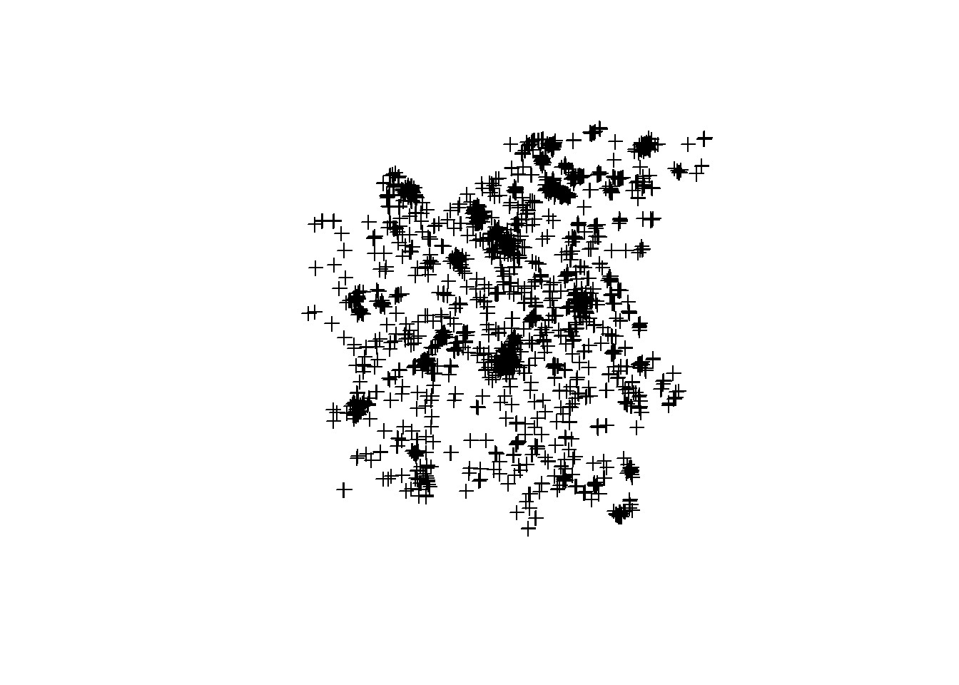
summary(wp_nonfunctional_sp)Object of class SpatialPoints
Coordinates:
min max
coords.x1 182490.7 291855.5
coords.x2 338261.8 448933.5
Is projected: TRUE
proj4string :
[+proj=tmerc +lat_0=4 +lon_0=4.5 +k=0.99975 +x_0=230738.26 +y_0=0
+a=6378249.145 +rf=293.465 +towgs84=-92,-93,122,0,0,0,0 +units=m
+no_defs]
Number of points: 2179Still using the as() function, we will be creating an owin object out of the nga_sp data frame. It is the perfect way to confine our analysis to the Osun State, Nigeria. As you may see next.
nga_owin <- as(nga_sp, "owin")
nga_owin
window: polygonal boundary
enclosing rectangle: [178398.73, 292278.89] x [329463.4, 452734.9] unitsplot(nga_owin)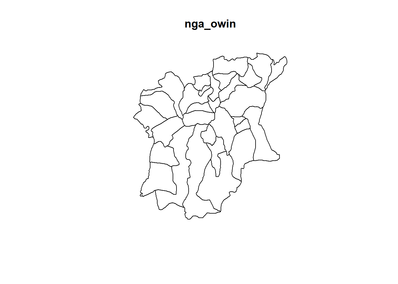
summary(nga_owin)Window: polygonal boundary
30 separate polygons (no holes)
vertices area relative.area
polygon 1 204 762071000 0.08870
polygon 2 81 302752000 0.03520
polygon 3 97 463731000 0.05400
polygon 4 124 371376000 0.04320
polygon 5 60 148866000 0.01730
polygon 6 84 144185000 0.01680
polygon 7 50 101744000 0.01180
polygon 8 72 214941000 0.02500
polygon 9 112 268551000 0.03120
polygon 10 125 363188000 0.04230
polygon 11 83 110665000 0.01290
polygon 12 126 191669000 0.02230
polygon 13 219 899941000 0.10500
polygon 14 174 737731000 0.08580
polygon 15 81 138238000 0.01610
polygon 16 65 118917000 0.01380
polygon 17 90 279120000 0.03250
polygon 18 69 69522200 0.00809
polygon 19 69 42545300 0.00495
polygon 20 49 30312400 0.00353
polygon 21 62 262061000 0.03050
polygon 22 93 436496000 0.05080
polygon 23 87 272566000 0.03170
polygon 24 105 507853000 0.05910
polygon 25 98 290780000 0.03380
polygon 26 64 325957000 0.03790
polygon 27 133 108439000 0.01260
polygon 28 122 460358000 0.05360
polygon 29 94 109183000 0.01270
polygon 30 95 60955300 0.00709
enclosing rectangle: [178398.73, 292278.89] x [329463.4, 452734.9] units
(113900 x 123300 units)
Window area = 8594710000 square units
Fraction of frame area: 0.612we shall end our geospatial data wrangling by extracting the functional and non-functional water points located within the Osun State in Nigeria. Using the code chunks below help us do that.
wp_functional_ppp = wp_functional_ppp[nga_owin]
plot(wp_functional_ppp)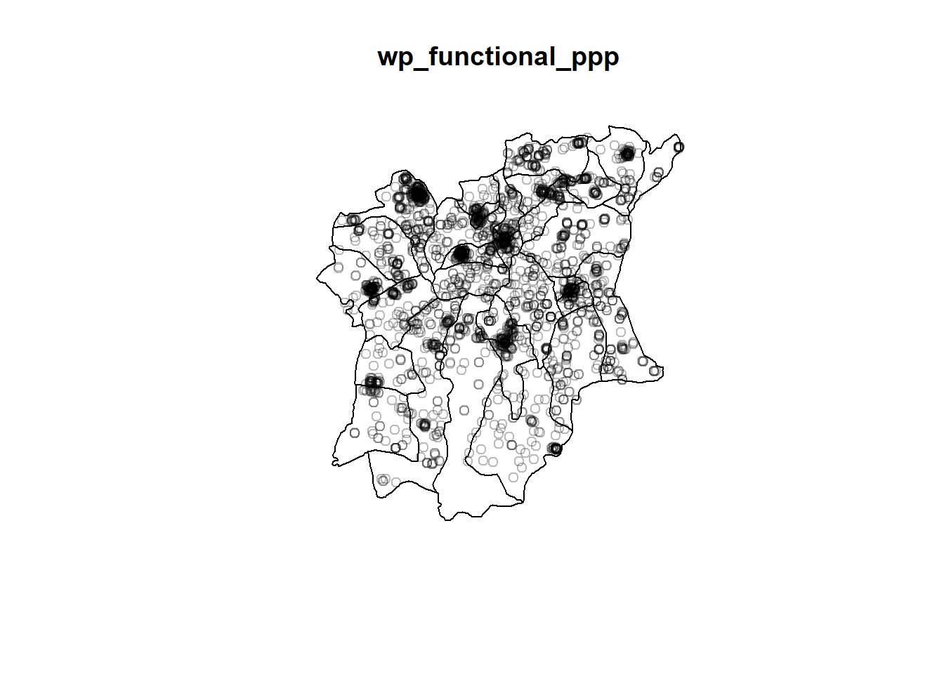
wp_nonfunctional_ppp = wp_nonfunctional_ppp[nga_owin]
plot(wp_nonfunctional_ppp)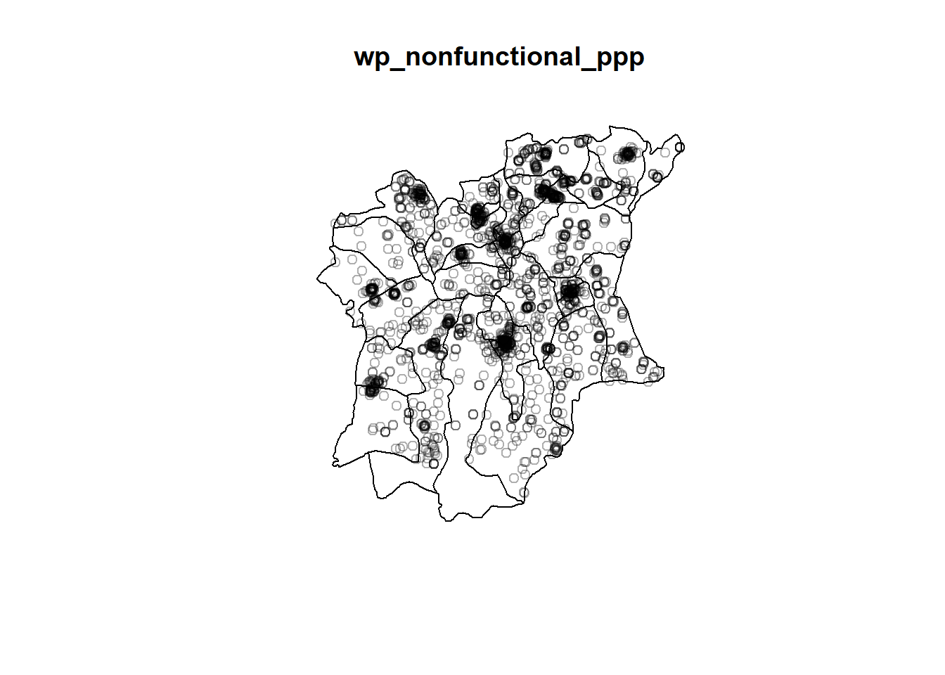
Looking at the plots above, we obtain two point maps with the water points located within the nga_owin object, so within the Osun State.
This section has for objective:
Deriving kernel density maps of functional and non-functional water points
Display kernel density maps of the Osun State, Nigeria on openstreetmap using appropriate tmap functions
Describe the spatial patterns revealed by the kernel density maps & highlight the advantage of kernel density map over point map
Our first step to KDE is to derive two density maps for functional and non-functional water points to check for any potential data problem. Here, we suspect that the scale of density values will be expressed in meters. The default measurement unit of Nigeria’s projected coordinate system – EPSG:26391 – is expressed in meters. We shall verify that and correct it to kilometers to get a more desirable map output (scale).
For starters, we should use the density() function to compute kernel density estimates for both types of water points. We will use two methods for smoothing the bandwidth for the kernel estimation point process intensity.
The first method uses adaptive estimate of the intensity function of a point pattern. We plot side-by-side the KDE maps for functional and non-functional WP.
kde_wpfunc.m <- adaptive.density(wp_functional_ppp,
                                  method = "kernel")

kde_wpnonfunc.m <- adaptive.density(wp_nonfunctional_ppp,
                                     method = "kernel")

par(mfrow=c(1,2))
plot(kde_wpfunc.m,
     main = "Functional Water Points",
     ribside=c("bottom"))
plot(kde_wpnonfunc.m,
     main = "Non-Functional Water Points",
     ribside=c("bottom"))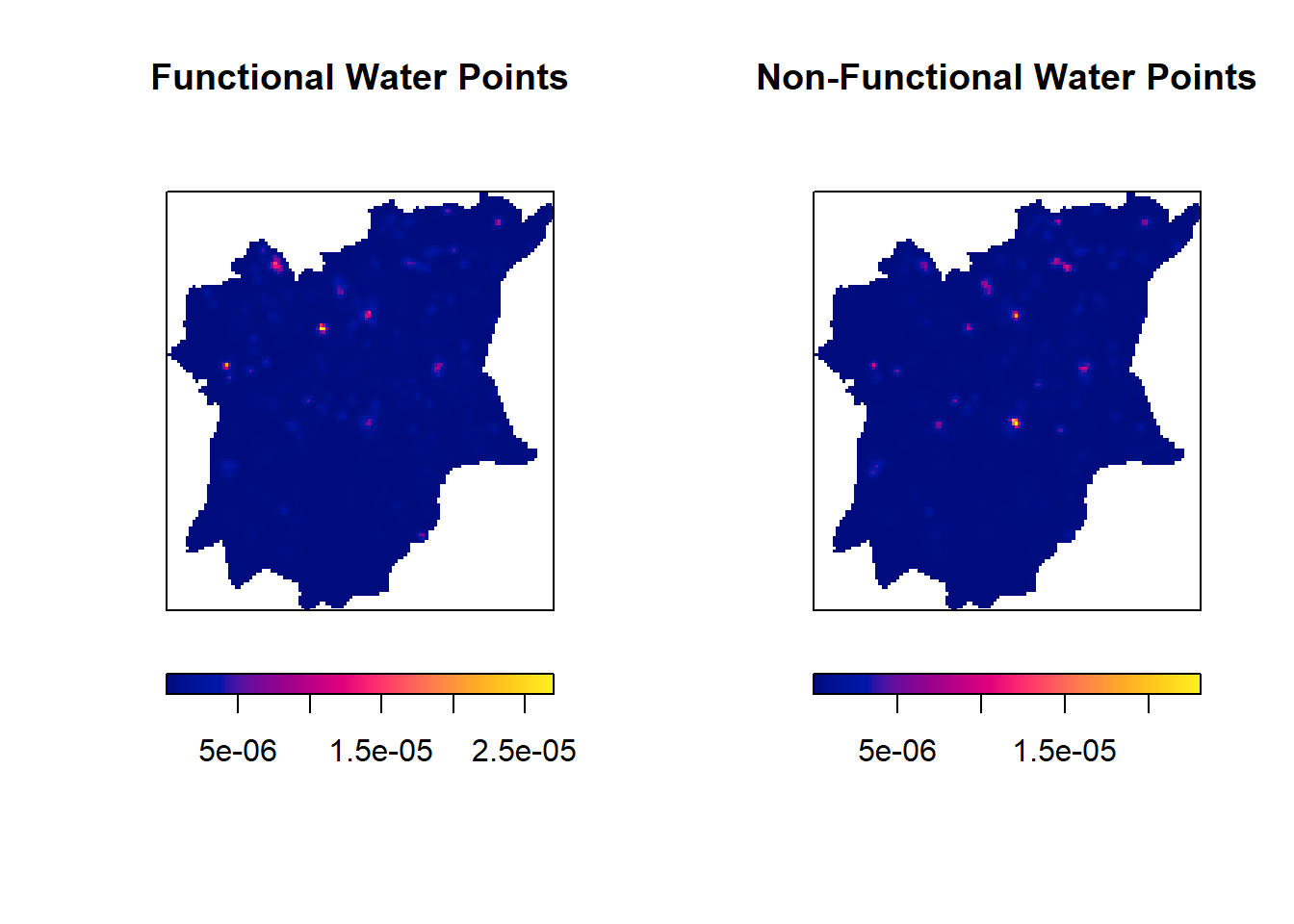
We observe potential clustering as some areas of the maps seem to have higher concentration of observations.
We also observe that the scale is set in meters, thus we will take action and re-scale our data points to kilometers.
Please find an alternative method for computing the bandwidth of our kernel density estimations.
kde_wpfunc.mppl <- density(wp_functional_ppp,
                               sigma=bw.ppl,
                               edge=TRUE)

kde_wpnonfunc.mppl <- density(wp_nonfunctional_ppp,
                             sigma=bw.ppl,
                             edge=TRUE)

par(mfrow=c(1,2))
plot(kde_wpfunc.mppl,
     main = "Functional Water Points",
     ribside=c("bottom"))
plot(kde_wpnonfunc.mppl,
     main = "Non-Functional Water Points",
     ribside=c("bottom"))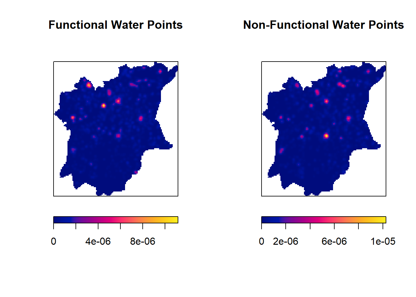
The density values of the output range from 0 to 0.000006 and it makes for an output difficult to comprehend and interpret. Thus, we will re-scale our density values to get an output in “number of points per square kilometer”.
To change the scale of the density values, we use the rescale() function from the spatstat.geom package. Here, we multiply values of our two objects of class ppp by 1000. We thus express them in kilometers and define the unit name to be “km”.
wp_functional_ppp.km <- rescale(wp_functional_ppp, 1000, "km")

wp_nonfunctional_ppp.km <- rescale(wp_nonfunctional_ppp, 1000, "km")
We can now run the previously used density() function using the re-scaled data and plot the output KDE map.
kde_wpfunc.km <- adaptive.density(wp_functional_ppp.km,
                                  method = "kernel")

kde_wpnonfunc.km <- adaptive.density(wp_nonfunctional_ppp.km,
                                     method = "kernel")

par(mfrow=c(1,2))
plot(kde_wpfunc.km,
     main = "Functional Water Points",
     ribside=c("bottom"))
plot(kde_wpnonfunc.km,
     main = "Non-Functional Water Points",
     ribside=c("bottom"))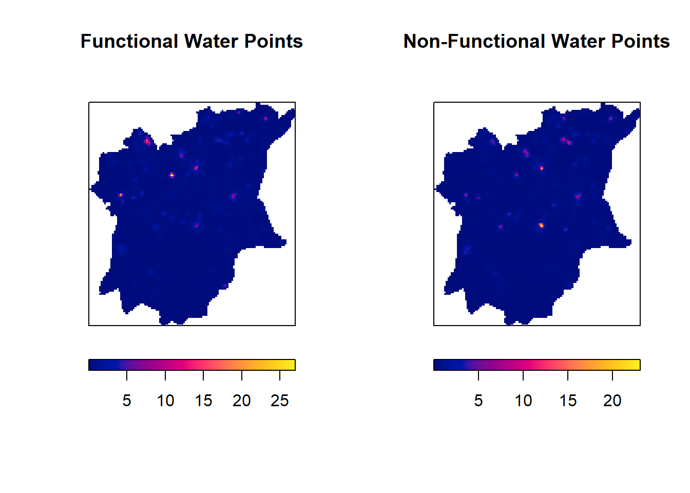
kde_wpfunc.ppl <- density(wp_functional_ppp.km,
                          sigma = bw.ppl,
                          edge = TRUE)

kde_wpnonfunc.ppl <- density(wp_nonfunctional_ppp.km,
                             sigma = bw.ppl,
                             edge = TRUE)

par(mfrow=c(1,2))
plot(kde_wpfunc.ppl,
     main = "Functional Water Points",
     ribside=c("bottom"))
plot(kde_wpnonfunc.ppl,
     main = "Non-Functional Water Points",
     ribside=c("bottom"))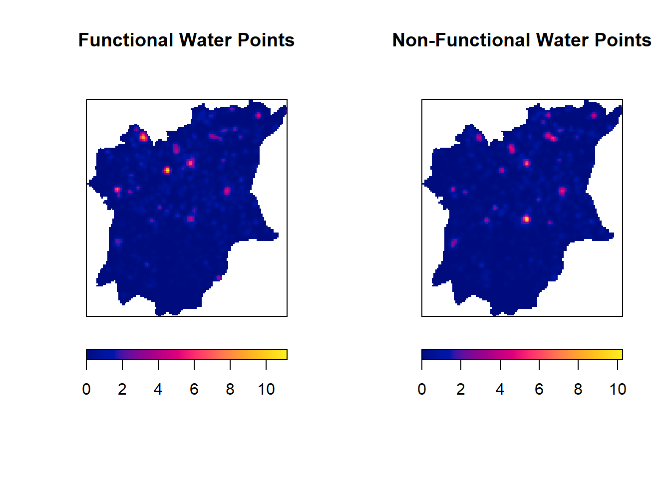
We start observing signs of potential clustering but, for now, we shall focus on transforming our im objects into rasters to plot our KDE maps using the tmap package. We will talk more about CSR and clustering later.
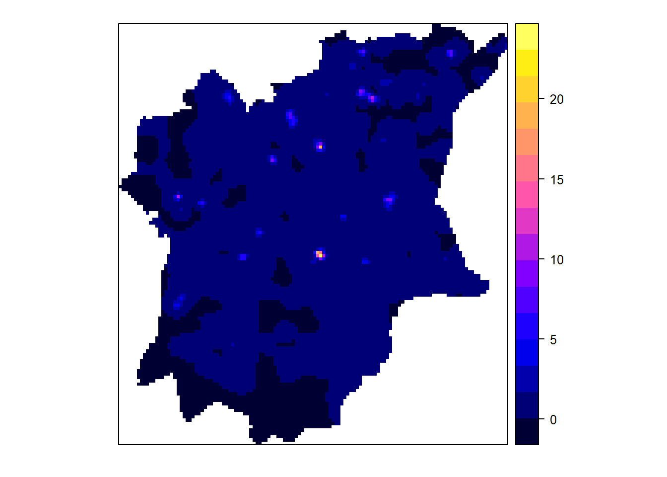
Here, we convert our KDE objects into grid objects for mapping purposes.
gridded_wpfunc <- as.SpatialGridDataFrame.im(kde_wpfunc.km)
gridded_wpnonfunc <- as.SpatialGridDataFrame.im(kde_wpnonfunc.km)

spplot(gridded_wpfunc)
spplot(gridded_wpnonfunc)
gridded_wpfunc.ppl <- as.SpatialGridDataFrame.im(kde_wpfunc.ppl)
gridded_wpnonfunc.ppl <- as.SpatialGridDataFrame.im(kde_wpnonfunc.ppl)

spplot(gridded_wpfunc.ppl)
spplot(gridded_wpnonfunc.ppl)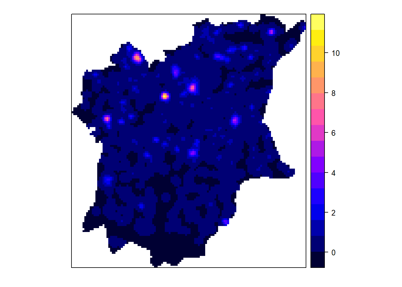

Now, we shall convert the gridded KDE objects into RasterLayer objects using the raster() function of the raster package. RasterLayer objects being compatible with the tmap functions, it allows us to plot our KDE map using OpenStreetView.
kde_wpfunc_raster <- raster(gridded_wpfunc)
kde_wpnonfunc_raster <- raster(gridded_wpnonfunc)

kde_wpfunc_raster
class : RasterLayer
dimensions : 128, 128, 16384 (nrow, ncol, ncell)
resolution : 0.8896887, 0.9630582 (x, y)
extent : 178.3987, 292.2789, 329.4634, 452.7349 (xmin, xmax, ymin, ymax)
crs : NA
source : memory
names : v
values : 1.702123e-16, 26.9948 (min, max)kde_wpnonfunc_rasterclass : RasterLayer
dimensions : 128, 128, 16384 (nrow, ncol, ncell)
resolution : 0.8896887, 0.9630582 (x, y)
extent : 178.3987, 292.2789, 329.4634, 452.7349 (xmin, xmax, ymin, ymax)
crs : NA
source : memory
names : v
values : 2.624981e-14, 23.06775 (min, max)Note that the CRS is NA.
kde_wpfunc_raster.ppl <- raster(gridded_wpfunc.ppl)
kde_wpnonfunc_raster.ppl <- raster(gridded_wpnonfunc.ppl)

kde_wpfunc_raster.ppl
class : RasterLayer
dimensions : 128, 128, 16384 (nrow, ncol, ncell)
resolution : 0.8896887, 0.9630582 (x, y)
extent : 178.3987, 292.2789, 329.4634, 452.7349 (xmin, xmax, ymin, ymax)
crs : NA
source : memory
names : v
values : -3.514656e-16, 11.15238 (min, max)kde_wpnonfunc_raster.pplclass : RasterLayer
dimensions : 128, 128, 16384 (nrow, ncol, ncell)
resolution : 0.8896887, 0.9630582 (x, y)
extent : 178.3987, 292.2789, 329.4634, 452.7349 (xmin, xmax, ymin, ymax)
crs : NA
source : memory
names : v
values : -3.628555e-16, 10.26005 (min, max)Note that the CRS is NA.
projection(kde_wpfunc_raster) <- CRS("+init=EPSG:26391 +datum:WGS84 +units=km")
projection(kde_wpfunc_raster.ppl) <- CRS("+init=EPSG:26391 +datum:WGS84 +units=km")

kde_wpfunc_raster
class : RasterLayer
dimensions : 128, 128, 16384 (nrow, ncol, ncell)
resolution : 0.8896887, 0.9630582 (x, y)
extent : 178.3987, 292.2789, 329.4634, 452.7349 (xmin, xmax, ymin, ymax)
crs : +init=EPSG:26391 +datum:WGS84 +units=km
source : memory
names : v
values : 1.702123e-16, 26.9948 (min, max)kde_wpfunc_raster.pplclass : RasterLayer
dimensions : 128, 128, 16384 (nrow, ncol, ncell)
resolution : 0.8896887, 0.9630582 (x, y)
extent : 178.3987, 292.2789, 329.4634, 452.7349 (xmin, xmax, ymin, ymax)
crs : +init=EPSG:26391 +datum:WGS84 +units=km
source : memory
names : v
values : -3.514656e-16, 11.15238 (min, max)projection(kde_wpnonfunc_raster) <- CRS("+init=EPSG:26391 +datum:WGS84 +units=km")
projection(kde_wpnonfunc_raster.ppl) <- CRS("+init=EPSG:26391 +datum:WGS84 +units=km")
kde_wpnonfunc_rasterclass : RasterLayer
dimensions : 128, 128, 16384 (nrow, ncol, ncell)
resolution : 0.8896887, 0.9630582 (x, y)
extent : 178.3987, 292.2789, 329.4634, 452.7349 (xmin, xmax, ymin, ymax)
crs : +init=EPSG:26391 +datum:WGS84 +units=km
source : memory
names : v
values : 2.624981e-14, 23.06775 (min, max)kde_wpnonfunc_raster.pplclass : RasterLayer
dimensions : 128, 128, 16384 (nrow, ncol, ncell)
resolution : 0.8896887, 0.9630582 (x, y)
extent : 178.3987, 292.2789, 329.4634, 452.7349 (xmin, xmax, ymin, ymax)
crs : +init=EPSG:26391 +datum:WGS84 +units=km
source : memory
names : v
values : -3.628555e-16, 10.26005 (min, max)Since we converted our KDE maps to raster objects, we will be able to plot the maps with the tmap package. Using the tm_basemap() function, we set OpenStreetMap as the default view mode on our interactive map. Then, using tm_shape() and tm_raster(), we plot the density estimates on the map and the Osun State layer.
tmap_mode('view')
tm_basemap("OpenStreetMap") +
tm_shape(kde_wpfunc_raster) +
tm_raster("v")tmap_mode('view')
tm_basemap("OpenStreetMap") +
tm_shape(kde_wpnonfunc_raster) +
tm_raster("v")tmap_mode("plot")The kernel density maps reveal locations with higher density of functional and non-functional water points. We observe density peaks of up to 27 functional water points and 23 non-functional water points.
It seems that we can observe clusters of functional and non-functional water points across the Osun state, however, this is just an intuition and it should be validated with further testing.
Looking back at the point maps and comparing with these new KDE maps, it seems obvious that the latter offers much better clarity in terms of interpretation. What appeared to look like strongly concentrated functional and non-functional water points on the lint map, now looks much neater and many of these zones disappear.
The KDE maps help us get a better understanding of the concentration and intensity. The point map gives us only a rough idea and no clear possible interpretation.
However, we should note that KDE maps are only good to display the data in an understandable manner. I believe that extra-work should be put into understanding what factors may explain the higher density zones and if there are any correlation between the location of functional and non-functional water points.
Before moving on to the Second-order Spatial Points Analysis, I would like to perform the Clark-Evans test to measure aggregation of functional and non-functional water points. The goal is to test the randomness of the data points and assess whether they are randomly distributed, clustered or dispersed.
We will perform a series of 2 tests, first on functional water points and, second, on non-functional water points. We will be using the clarkevans.test() function of the spatstat package.
The hypotheses are the following:
Test 1
H0 : Functional Water Points are randomly distributed
H1 : Functional Water Points are not randomly distributed, they are clustered
Test 2
H0 : Non-functional Water Points are randomly distributed
H1 : Non-functional Water Points are not randomly distributed, they are clustered
As you may have read above, we determine the alternative hypothesis to be that water points are clustered. This decision is based on an intuition that derives from the previously seen visual representations of functional and non-functional water points. Indeed, we observed in our KDE plots some concentration of data points across the Osun State. Thus, we would like to test for clustering directly to prove this intuition.
Please note that when conducting our tests, we will use a 5% significance level.
First test on functional water points.
clarkevans.test(wp_functional_ppp,
                correction="none",
                clipregion=NULL,
                alternative=c("clustered"),
                nsim=99)
    Clark-Evans test
    No edge correction
    Monte Carlo test based on 99 simulations of CSR with fixed n

data:  wp_functional_ppp
R = 0.44265, p-value = 0.01
alternative hypothesis: clustered (R < 1)
Second test on non-functional water points
clarkevans.test(wp_nonfunctional_ppp,
                correction="none",
                clipregion=NULL,
                alternative=c("clustered"),
                nsim=99)
    Clark-Evans test
    No edge correction
    Monte Carlo test based on 99 simulations of CSR with fixed n

data:  wp_nonfunctional_ppp
R = 0.43223, p-value = 0.01
alternative hypothesis: clustered (R < 1)Since both p-values of the respective tests (0.01 and 0.01) are below the significance level and that the R-values are below 1, we reject the null hypothesis suggesting that functional and non-functional water points are clustered. Note that this is just a preliminary test and that we shall confirm this conclusion using second-order spatial point patterns analysis methods.
For the purpose of our second-order SPPA, we will use the L function using Lest() of the spatstat package. Most importantly, we will perform Monte-Carlo simulation tests using the envelope() function of spatstat.
Note that it requires a lot of computation power to perform the Monte-Carlo simulations. Therefore, to run the code faster, we will be performing tests for all level-2 administrative zones separately.
H0 : Functional Water Points are randomly distributed
H1 : Functional Water Points are not randomly distributed
We will be using a 5% significance level in our tests. By doing so, we will be running 40 Monte-Carlo simulations and it should contribute to making the code easier to run.
This first piece of code you can find just below is the code you would use to perform a single analysis for Functional Water Points in the case of the code chunk below.
L_wpfunc = Lest(wp_functional_ppp, correction = "Ripley")
plot(L_wpfunc, . -r ~ r, ylab= "L(d)-r", xlab = "d(m)")
This second piece of code is the one you would use to perform a Monte-Carlo simulation on Functional Water Points in the Osun State of Nigeria. As explained, the computational power of my laptop does not allow me to run the code chunk in a reasonable amount of time, so I will be doing Admin Level-2 boudary analysis.
L_wp1.csr <- envelope(wp_functional_ppp, Lest, nsim = 39, rank = 1, glocal=TRUE)
plot(L_wp1.csr, . - r ~ r, xlab="d", ylab="L(d)-r", main = "L-test for Functional Water Points in Osun State")for (i in 1:30){
print(paste("Test", i))
print(paste("Now analyzing Administrative Level-2:", nga$ADM2_EN[i]))
nga1 = nga[i,]
nga_spat = as_Spatial(nga1)
nga_sp = as(nga_spat, "SpatialPolygons")
nga_owin = as(nga_sp, "owin")
wp_functional_R = wp_functional_ppp[nga_owin]
L_wp1.csr <- envelope(wp_functional_R, Lest, nsim = 39, rank = 1, glocal=TRUE)
title = paste("L-test for Functional Water Points in", nga$ADM2_EN[i])
plot(L_wp1.csr, . - r ~ r, xlab="d", ylab="L(d)-r", main = title)
print("—————————————————————————————————————————————————————————————————————")
}[1] "Test 1"
[1] "Now analyzing Administrative Level-2: Aiyedade"
Generating 39 simulations of CSR ...
1, 2, 3, 4, 5, 6, 7, 8, 9, 10, 11, 12, 13, 14, 15, 16, 17, 18, 19, 20, 21, 22, 23, 24, 25, 26, 27, 28, 29, 30, 31, 32, 33, 34, 35, 36, 37, 38, 39.
Done.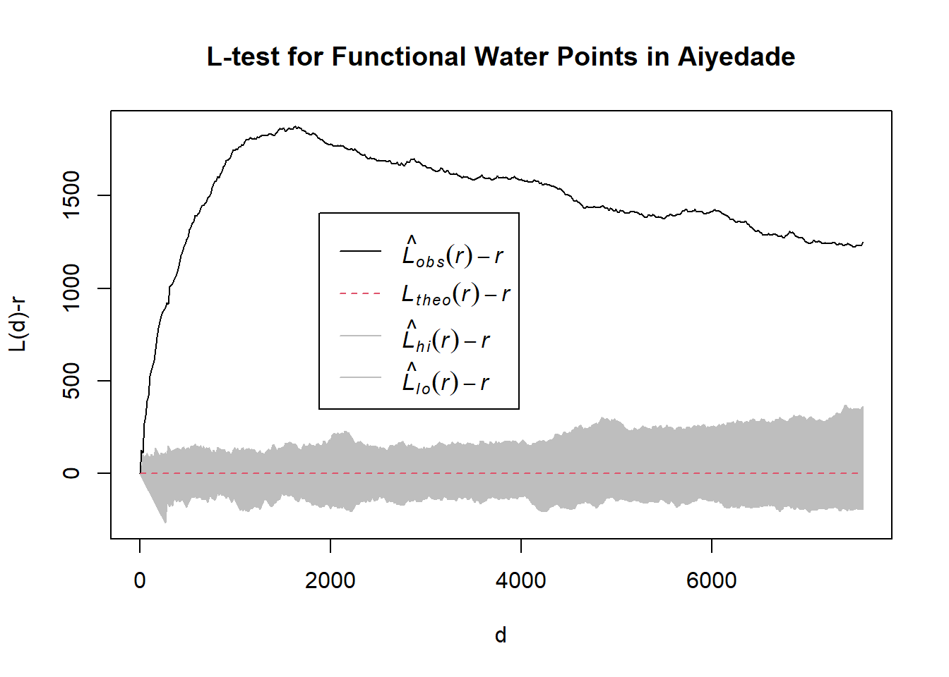
[1] "—————————————————————————————————————————————————————————————————————"
[1] "Test 2"
[1] "Now analyzing Administrative Level-2: Aiyedire"
Generating 39 simulations of CSR  ...
1, 2, 3, 4, 5, 6, 7, 8, 9, 10, 11, 12, 13, 14, 15, 16, 17, 18, 19, 20, 21, 22, 23, 24, 25, 26, 27, 28, 29, 30, 31, 32, 33, 34, 35, 36, 37, 38,  39.

Done.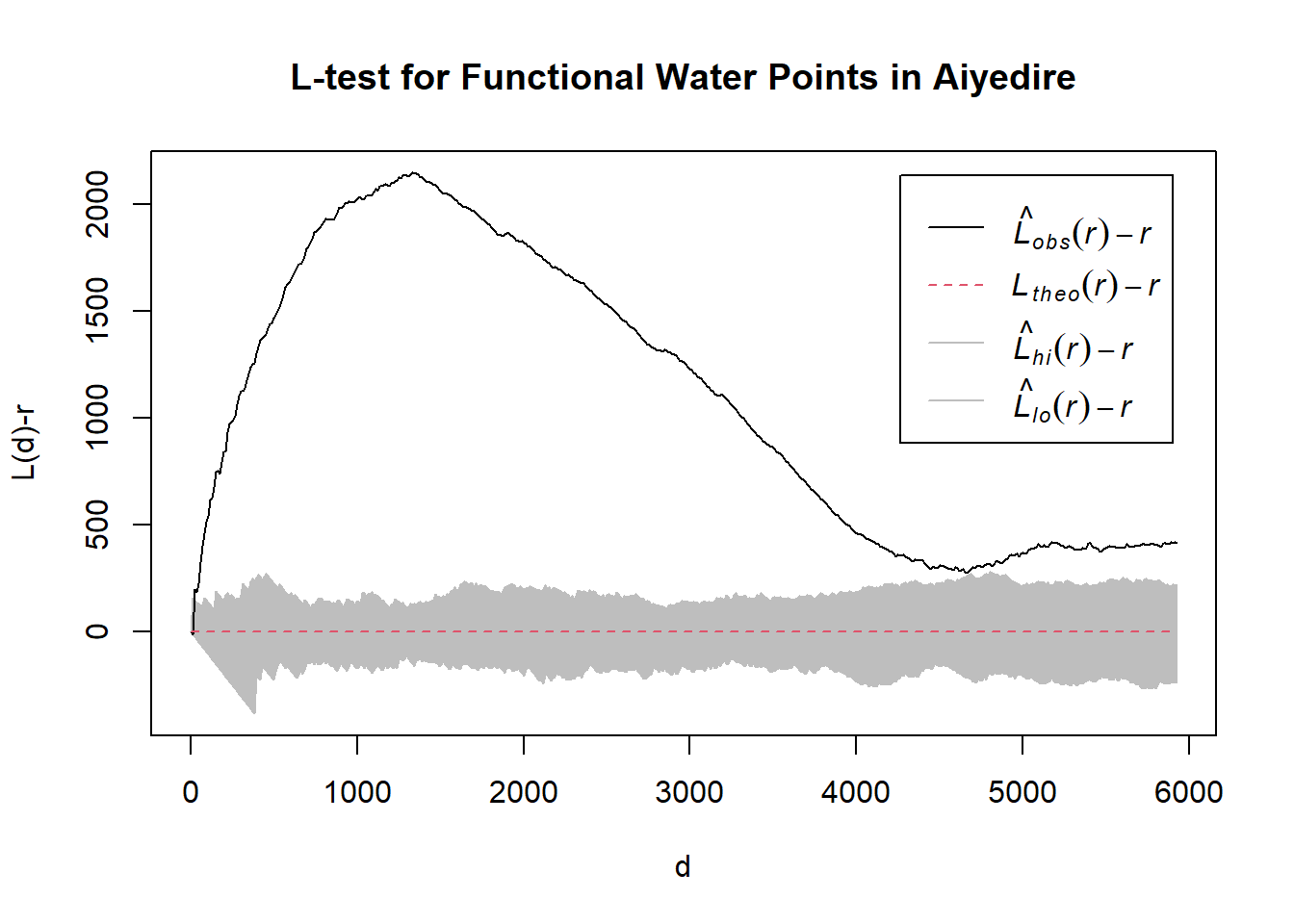
[1] "—————————————————————————————————————————————————————————————————————"
[1] "Test 3"
[1] "Now analyzing Administrative Level-2: Atakumosa East"
Generating 39 simulations of CSR  ...
1, 2, 3, 4, 5, 6, 7, 8, 9, 10, 11, 12, 13, 14, 15, 16, 17, 18, 19, 20, 21, 22, 23, 24, 25, 26, 27, 28, 29, 30, 31, 32, 33, 34, 35, 36, 37, 38,  39.

Done.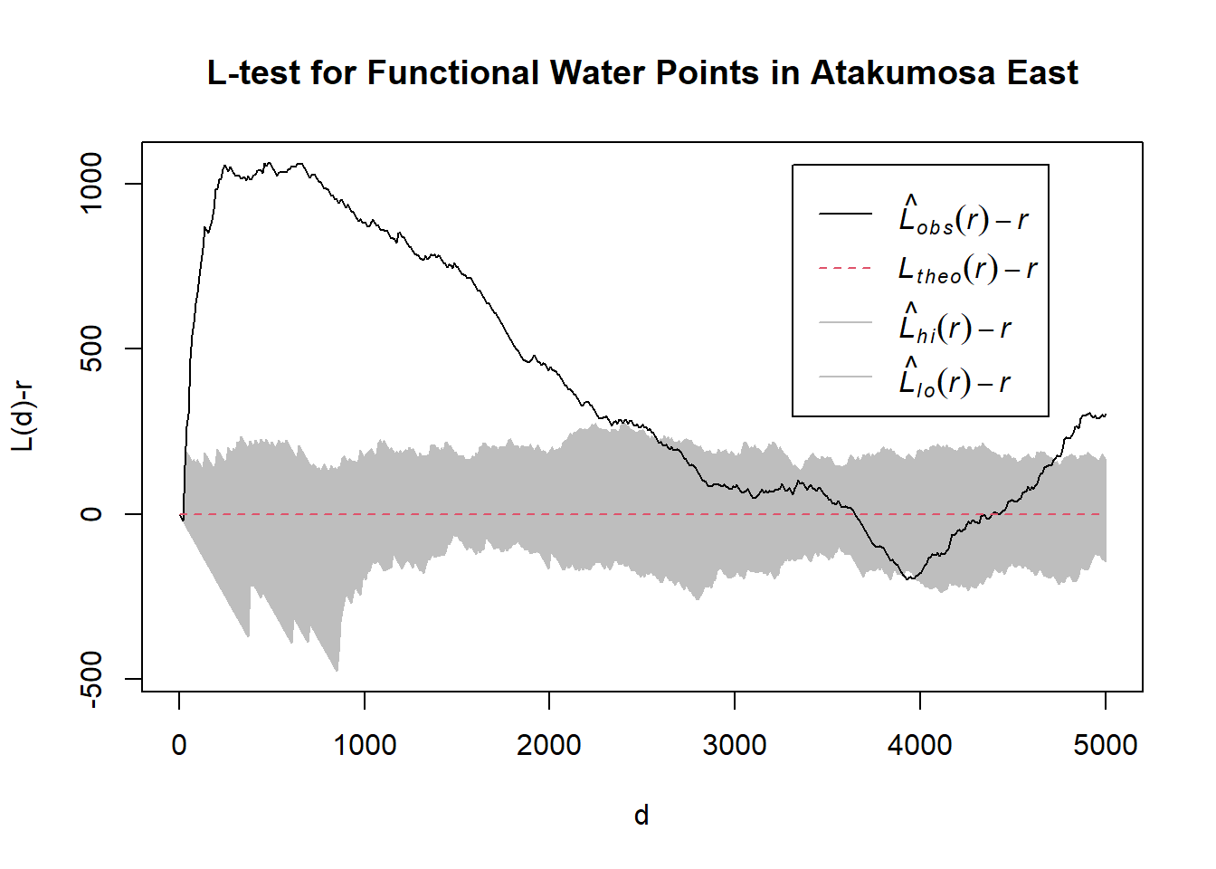
[1] "—————————————————————————————————————————————————————————————————————"
[1] "Test 4"
[1] "Now analyzing Administrative Level-2: Atakumosa West"
Generating 39 simulations of CSR  ...
1, 2, 3, 4, 5, 6, 7, 8, 9, 10, 11, 12, 13, 14, 15, 16, 17, 18, 19, 20, 21, 22, 23, 24, 25, 26, 27, 28, 29, 30, 31, 32, 33, 34, 35, 36, 37, 38,  39.

Done.
[1] "—————————————————————————————————————————————————————————————————————"
[1] "Test 5"
[1] "Now analyzing Administrative Level-2: Boluwaduro"
Generating 39 simulations of CSR  ...
1, 2, 3, 4, 5, 6, 7, 8, 9, 10, 11, 12, 13, 14, 15, 16, 17, 18, 19, 20, 21, 22, 23, 24, 25, 26, 27, 28, 29, 30, 31, 32, 33, 34, 35, 36, 37, 38,  39.

Done.
[1] "—————————————————————————————————————————————————————————————————————"
[1] "Test 6"
[1] "Now analyzing Administrative Level-2: Boripe"
Generating 39 simulations of CSR  ...
1, 2, 3, 4, 5, 6, 7, 8, 9, 10, 11, 12, 13, 14, 15, 16, 17, 18, 19, 20, 21, 22, 23, 24, 25, 26, 27, 28, 29, 30, 31, 32, 33, 34, 35, 36, 37, 38,  39.

Done.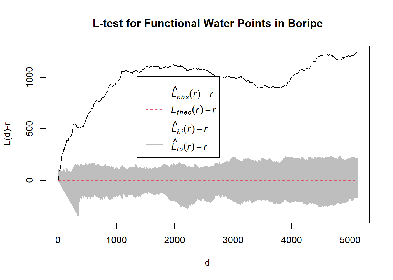
[1] "—————————————————————————————————————————————————————————————————————"
[1] "Test 7"
[1] "Now analyzing Administrative Level-2: Ede North"
Generating 39 simulations of CSR  ...
1, 2, 3, 4, 5, 6, 7, 8, 9, 10, 11, 12, 13, 14, 15, 16, 17, 18, 19, 20, 21, 22, 23, 24, 25, 26, 27, 28, 29, 30, 31, 32, 33, 34, 35, 36, 37, 38,  39.

Done.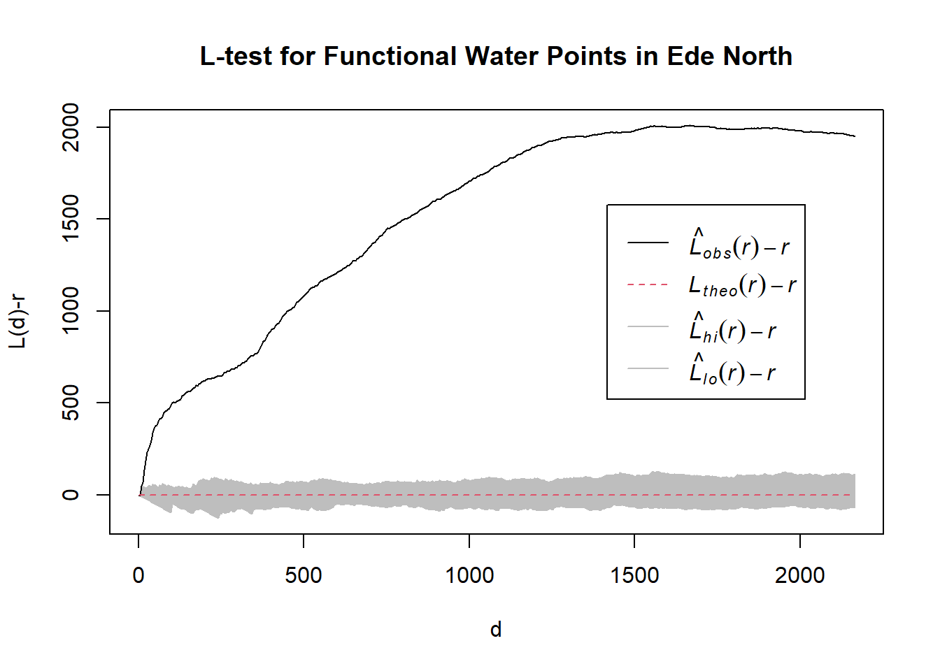
[1] "—————————————————————————————————————————————————————————————————————"
[1] "Test 8"
[1] "Now analyzing Administrative Level-2: Ede South"
Generating 39 simulations of CSR  ...
1, 2, 3, 4, 5, 6, 7, 8, 9, 10, 11, 12, 13, 14, 15, 16, 17, 18, 19, 20, 21, 22, 23, 24, 25, 26, 27, 28, 29, 30, 31, 32, 33, 34, 35, 36, 37, 38,  39.

Done.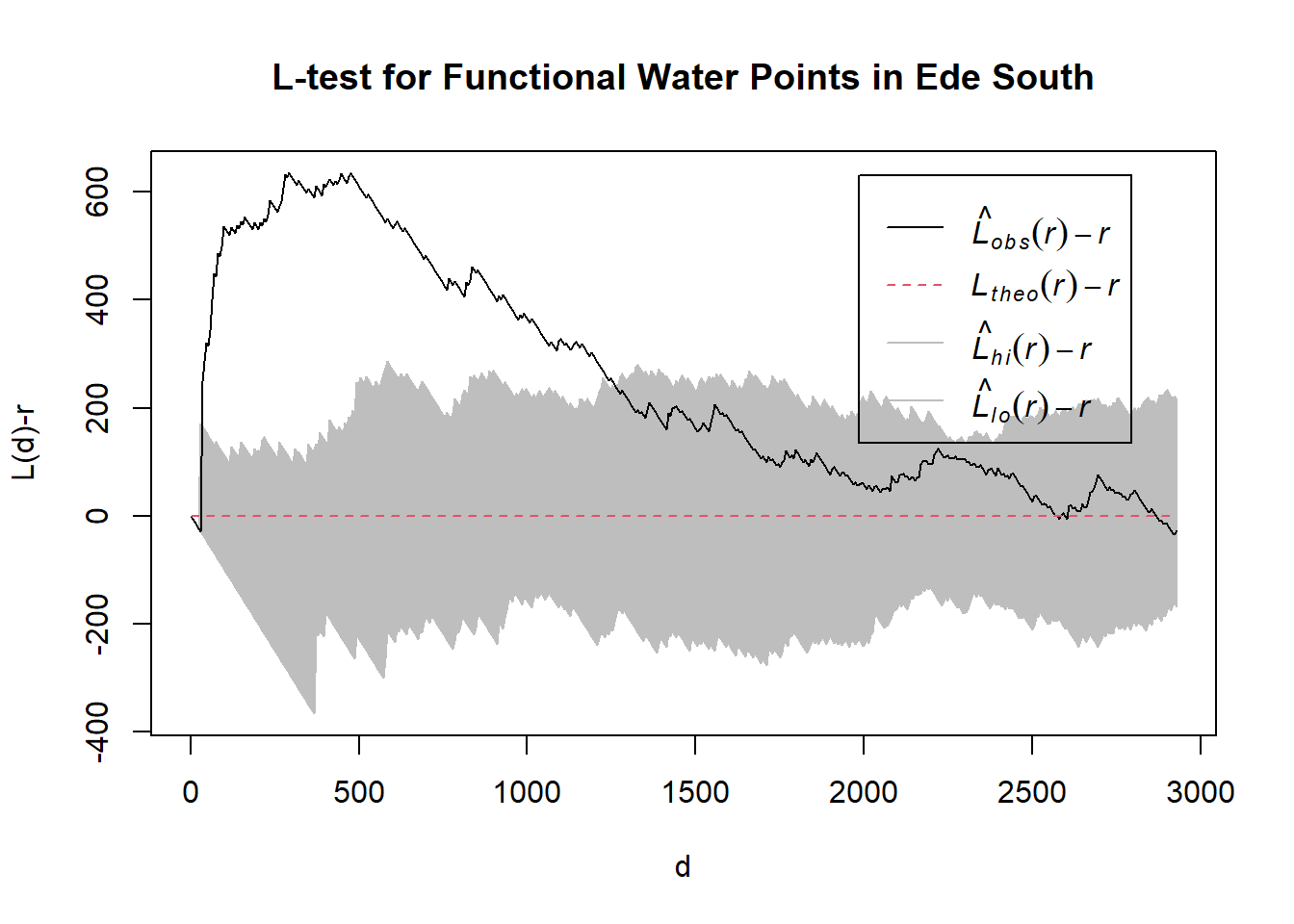
[1] "—————————————————————————————————————————————————————————————————————"
[1] "Test 9"
[1] "Now analyzing Administrative Level-2: Egbedore"
Generating 39 simulations of CSR  ...
1, 2, 3, 4, 5, 6, 7, 8, 9, 10, 11, 12, 13, 14, 15, 16, 17, 18, 19, 20, 21, 22, 23, 24, 25, 26, 27, 28, 29, 30, 31, 32, 33, 34, 35, 36, 37, 38,  39.

Done.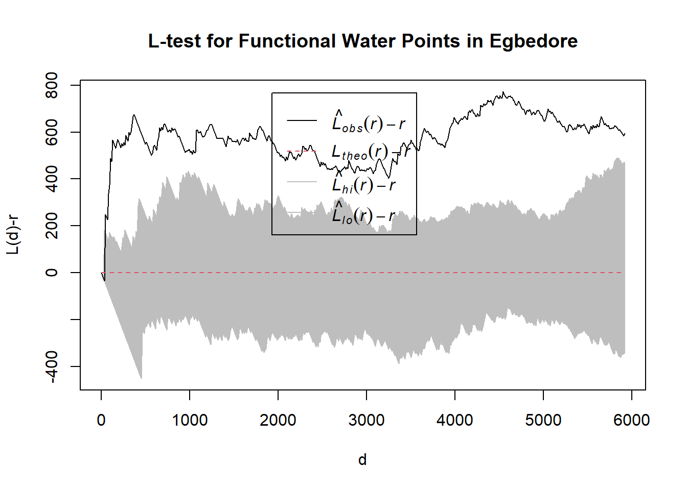
[1] "—————————————————————————————————————————————————————————————————————"
[1] "Test 10"
[1] "Now analyzing Administrative Level-2: Ejigbo"
Generating 39 simulations of CSR  ...
1, 2, 3, 4, 5, 6, 7, 8, 9, 10, 11, 12, 13, 14, 15, 16, 17, 18, 19, 20, 21, 22, 23, 24, 25, 26, 27, 28, 29, 30, 31, 32, 33, 34, 35, 36, 37, 38,  39.

Done.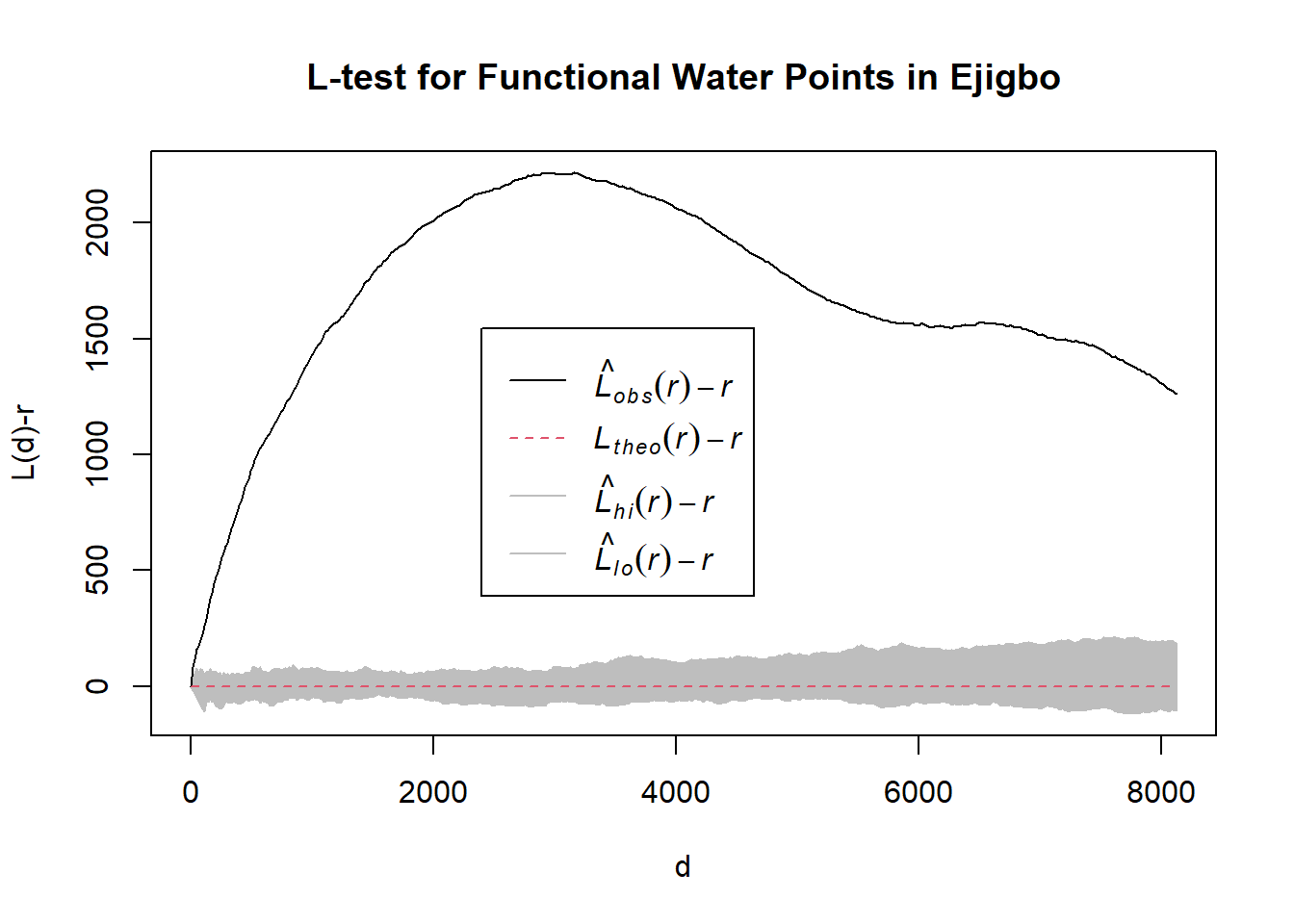
[1] "—————————————————————————————————————————————————————————————————————"
[1] "Test 11"
[1] "Now analyzing Administrative Level-2: Ife Central"
Generating 39 simulations of CSR  ...
1, 2, 3, 4, 5, 6, 7, 8, 9, 10, 11, 12, 13, 14, 15, 16, 17, 18, 19, 20, 21, 22, 23, 24, 25, 26, 27, 28, 29, 30, 31, 32, 33, 34, 35, 36, 37, 38,  39.

Done.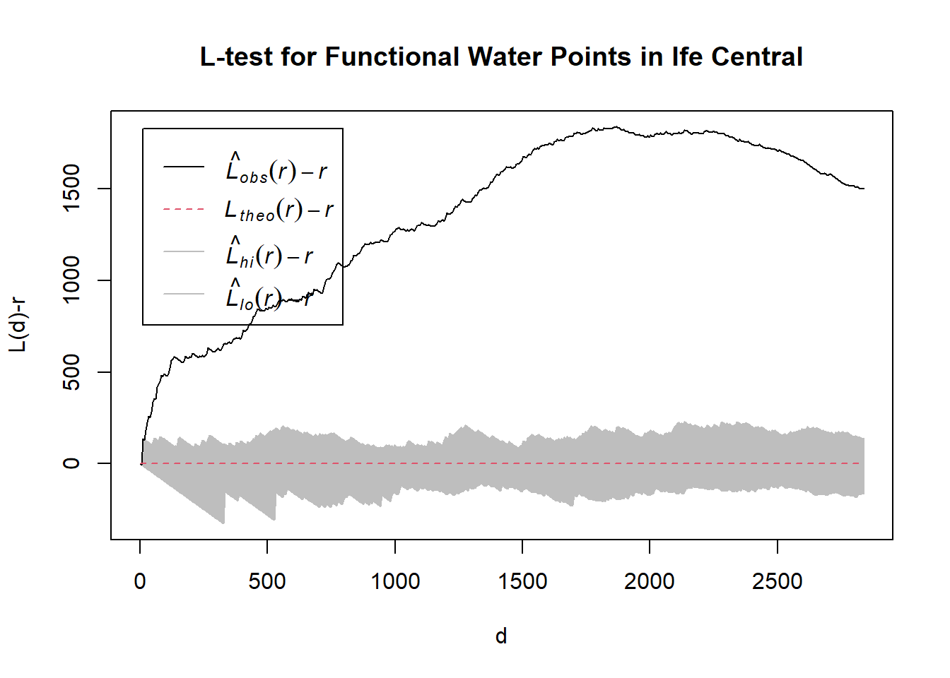
[1] "—————————————————————————————————————————————————————————————————————"
[1] "Test 12"
[1] "Now analyzing Administrative Level-2: Ife East"
Generating 39 simulations of CSR  ...
1, 2, 3, 4, 5, 6, 7, 8, 9, 10, 11, 12, 13, 14, 15, 16, 17, 18, 19, 20, 21, 22, 23, 24, 25, 26, 27, 28, 29, 30, 31, 32, 33, 34, 35, 36, 37, 38,  39.

Done.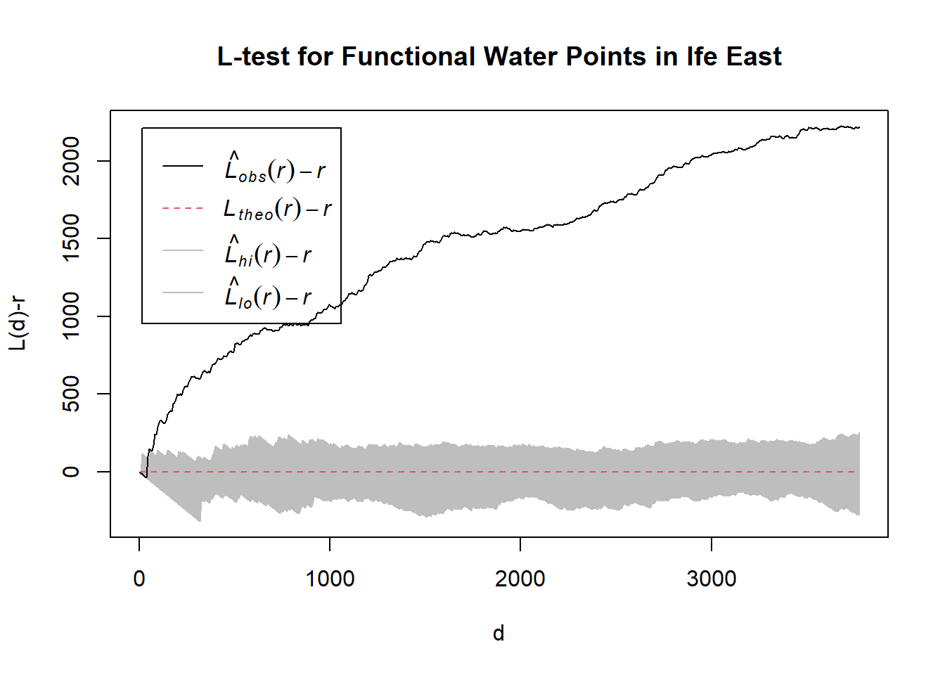
[1] "—————————————————————————————————————————————————————————————————————"
[1] "Test 13"
[1] "Now analyzing Administrative Level-2: Ife North"
Generating 39 simulations of CSR  ...
1, 2, 3, 4, 5, 6, 7, 8, 9, 10, 11, 12, 13, 14, 15, 16, 17, 18, 19, 20, 21, 22, 23, 24, 25, 26, 27, 28, 29, 30, 31, 32, 33, 34, 35, 36, 37, 38,  39.

Done.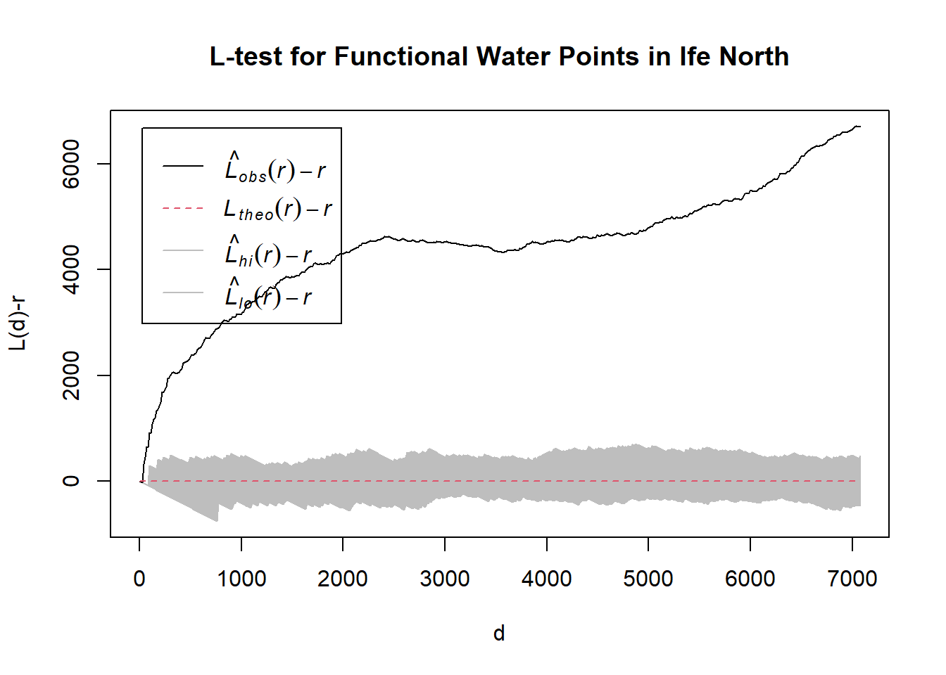
[1] "—————————————————————————————————————————————————————————————————————"
[1] "Test 14"
[1] "Now analyzing Administrative Level-2: Ife South"
Generating 39 simulations of CSR  ...
1, 2, 3, 4, 5, 6, 7, 8, 9, 10, 11, 12, 13, 14, 15, 16, 17, 18, 19, 20, 21, 22, 23, 24, 25, 26, 27, 28, 29, 30, 31, 32, 33, 34, 35, 36, 37, 38,  39.

Done.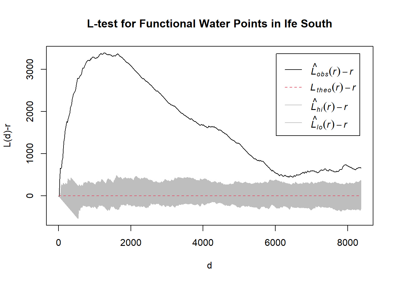
[1] "—————————————————————————————————————————————————————————————————————"
[1] "Test 15"
[1] "Now analyzing Administrative Level-2: Ifedayo"
Generating 39 simulations of CSR  ...
1, 2, 3, 4, 5, 6, 7, 8, 9, 10, 11, 12, 13, 14, 15, 16, 17, 18, 19, 20, 21, 22, 23, 24, 25, 26, 27, 28, 29, 30, 31, 32, 33, 34, 35, 36, 37, 38,  39.

Done.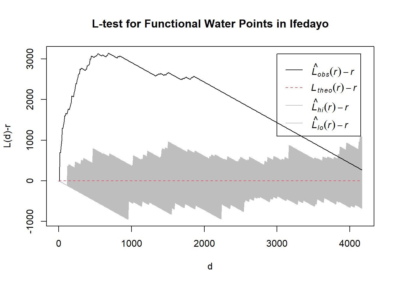
[1] "—————————————————————————————————————————————————————————————————————"
[1] "Test 16"
[1] "Now analyzing Administrative Level-2: Ifelodun"
Generating 39 simulations of CSR  ...
1, 2, 3, 4, 5, 6, 7, 8, 9, 10, 11, 12, 13, 14, 15, 16, 17, 18, 19, 20, 21, 22, 23, 24, 25, 26, 27, 28, 29, 30, 31, 32, 33, 34, 35, 36, 37, 38,  39.

Done.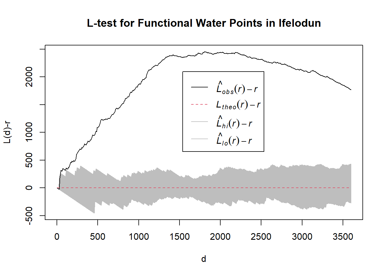
[1] "—————————————————————————————————————————————————————————————————————"
[1] "Test 17"
[1] "Now analyzing Administrative Level-2: Ila"
Generating 39 simulations of CSR  ...
1, 2, 3, 4, 5, 6, 7, 8, 9, 10, 11, 12, 13, 14, 15, 16, 17, 18, 19, 20, 21, 22, 23, 24, 25, 26, 27, 28, 29, 30, 31, 32, 33, 34, 35, 36, 37, 38,  39.

Done.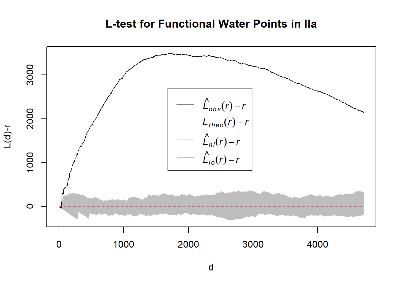
[1] "—————————————————————————————————————————————————————————————————————"
[1] "Test 18"
[1] "Now analyzing Administrative Level-2: Ilesha East"
Generating 39 simulations of CSR  ...
1, 2, 3, 4, 5, 6, 7, 8, 9, 10, 11, 12, 13, 14, 15, 16, 17, 18, 19, 20, 21, 22, 23, 24, 25, 26, 27, 28, 29, 30, 31, 32, 33, 34, 35, 36, 37, 38,  39.

Done.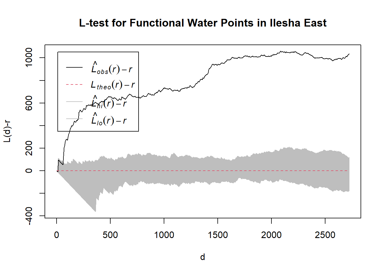
[1] "—————————————————————————————————————————————————————————————————————"
[1] "Test 19"
[1] "Now analyzing Administrative Level-2: Ilesha West"
Generating 39 simulations of CSR  ...
1, 2, 3, 4, 5, 6, 7, 8, 9, 10, 11, 12, 13, 14, 15, 16, 17, 18, 19, 20, 21, 22, 23, 24, 25, 26, 27, 28, 29, 30, 31, 32, 33, 34, 35, 36, 37, 38,  39.

Done.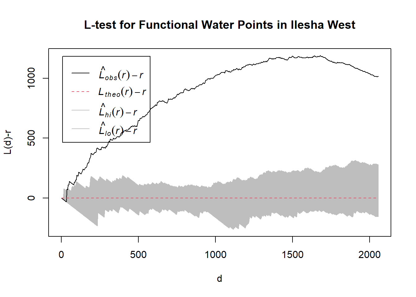
[1] "—————————————————————————————————————————————————————————————————————"
[1] "Test 20"
[1] "Now analyzing Administrative Level-2: Irepodun"
Generating 39 simulations of CSR  ...
1, 2, 3, 4, 5, 6, 7, 8, 9, 10, 11, 12, 13, 14, 15, 16, 17, 18, 19, 20, 21, 22, 23, 24, 25, 26, 27, 28, 29, 30, 31, 32, 33, 34, 35, 36, 37, 38,  39.

Done.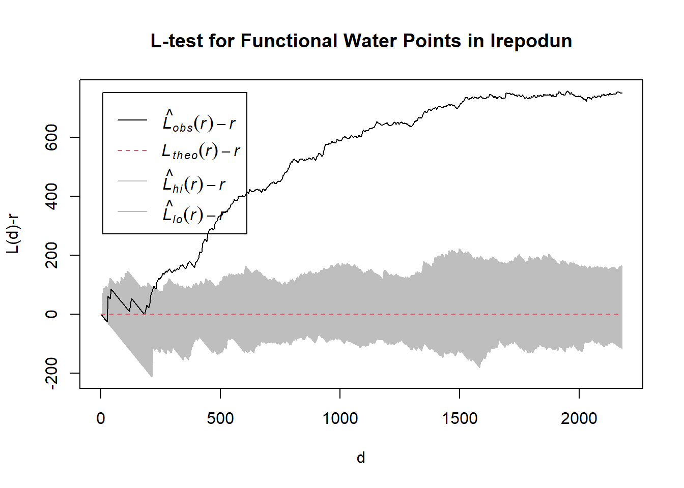
[1] "—————————————————————————————————————————————————————————————————————"
[1] "Test 21"
[1] "Now analyzing Administrative Level-2: Irewole"
Generating 39 simulations of CSR  ...
1, 2, 3, 4, 5, 6, 7, 8, 9, 10, 11, 12, 13, 14, 15, 16, 17, 18, 19, 20, 21, 22, 23, 24, 25, 26, 27, 28, 29, 30, 31, 32, 33, 34, 35, 36, 37, 38,  39.

Done.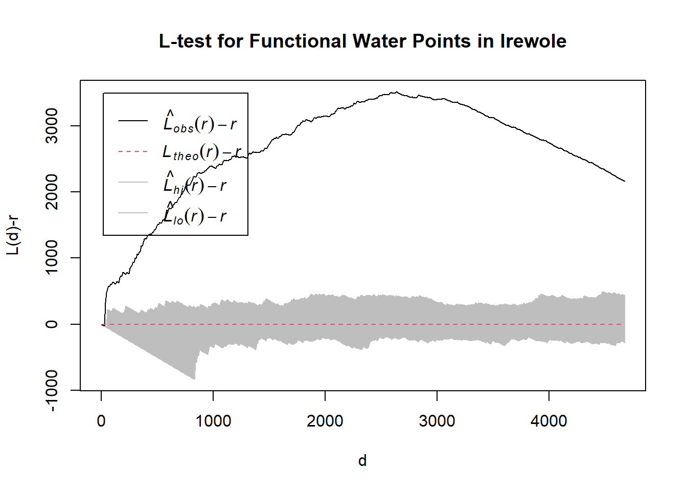
[1] "—————————————————————————————————————————————————————————————————————"
[1] "Test 22"
[1] "Now analyzing Administrative Level-2: Isokan"
Generating 39 simulations of CSR  ...
1, 2, 3, 4, 5, 6, 7, 8, 9, 10, 11, 12, 13, 14, 15, 16, 17, 18, 19, 20, 21, 22, 23, 24, 25, 26, 27, 28, 29, 30, 31, 32, 33, 34, 35, 36, 37, 38,  39.

Done.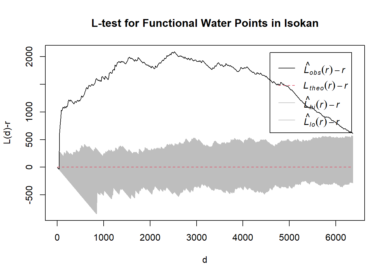
[1] "—————————————————————————————————————————————————————————————————————"
[1] "Test 23"
[1] "Now analyzing Administrative Level-2: Iwo"
Generating 39 simulations of CSR  ...
1, 2, 3, 4, 5, 6, 7, 8, 9, 10, 11, 12, 13, 14, 15, 16, 17, 18, 19, 20, 21, 22, 23, 24, 25, 26, 27, 28, 29, 30, 31, 32, 33, 34, 35, 36, 37, 38,  39.

Done.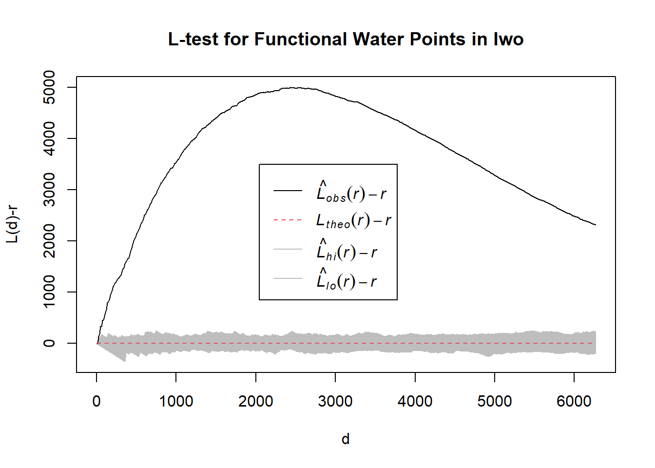
[1] "—————————————————————————————————————————————————————————————————————"
[1] "Test 24"
[1] "Now analyzing Administrative Level-2: Obokun"
Generating 39 simulations of CSR  ...
1, 2, 3, 4, 5, 6, 7, 8, 9, 10, 11, 12, 13, 14, 15, 16, 17, 18, 19, 20, 21, 22, 23, 24, 25, 26, 27, 28, 29, 30, 31, 32, 33, 34, 35, 36, 37, 38,  39.

Done.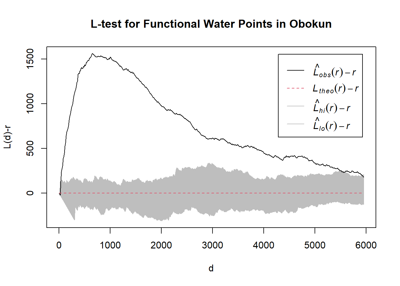
[1] "—————————————————————————————————————————————————————————————————————"
[1] "Test 25"
[1] "Now analyzing Administrative Level-2: Odo-Otin"
Generating 39 simulations of CSR  ...
1, 2, 3, 4, 5, 6, 7, 8, 9, 10, 11, 12, 13, 14, 15, 16, 17, 18, 19, 20, 21, 22, 23, 24, 25, 26, 27, 28, 29, 30, 31, 32, 33, 34, 35, 36, 37, 38,  39.

Done.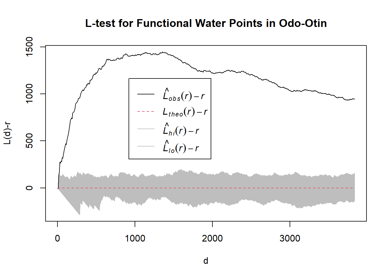
[1] "—————————————————————————————————————————————————————————————————————"
[1] "Test 26"
[1] "Now analyzing Administrative Level-2: Ola-oluwa"
Generating 39 simulations of CSR  ...
1, 2, 3, 4, 5, 6, 7, 8, 9, 10, 11, 12, 13, 14, 15, 16, 17, 18, 19, 20, 21, 22, 23, 24, 25, 26, 27, 28, 29, 30, 31, 32, 33, 34, 35, 36, 37, 38,  39.

Done.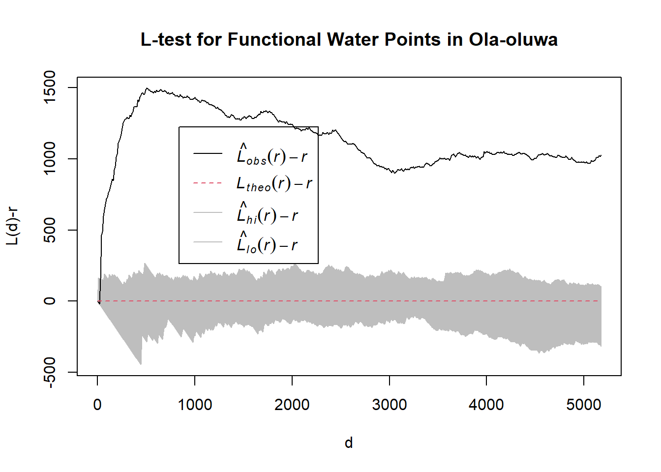
[1] "—————————————————————————————————————————————————————————————————————"
[1] "Test 27"
[1] "Now analyzing Administrative Level-2: Olorunda"
Generating 39 simulations of CSR  ...
1, 2, 3, 4, 5, 6, 7, 8, 9, 10, 11, 12, 13, 14, 15, 16, 17, 18, 19, 20, 21, 22, 23, 24, 25, 26, 27, 28, 29, 30, 31, 32, 33, 34, 35, 36, 37, 38,  39.

Done.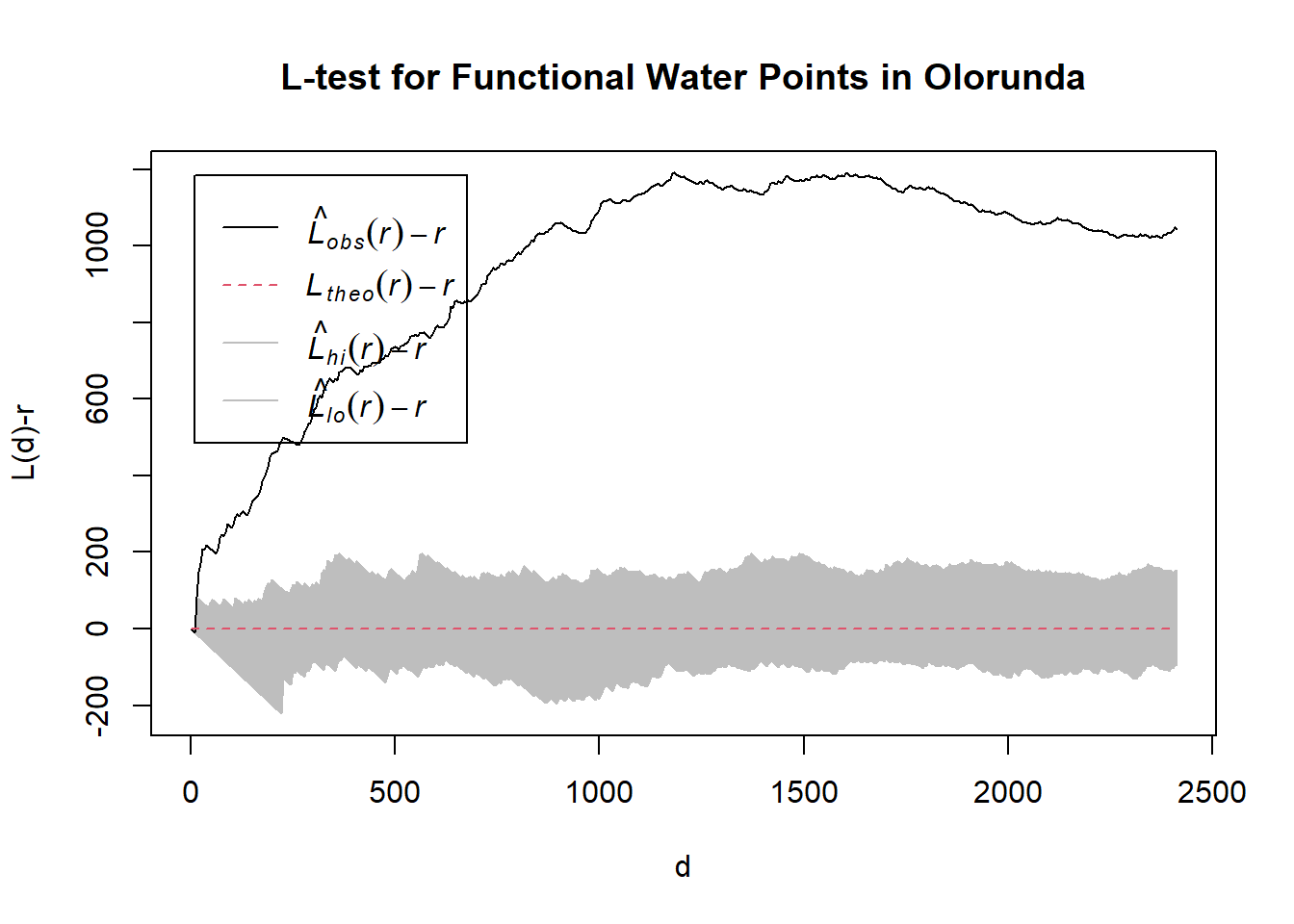
[1] "—————————————————————————————————————————————————————————————————————"
[1] "Test 28"
[1] "Now analyzing Administrative Level-2: Oriade"
Generating 39 simulations of CSR  ...
1, 2, 3, 4, 5, 6, 7, 8, 9, 10, 11, 12, 13, 14, 15, 16, 17, 18, 19, 20, 21, 22, 23, 24, 25, 26, 27, 28, 29, 30, 31, 32, 33, 34, 35, 36, 37, 38,  39.

Done.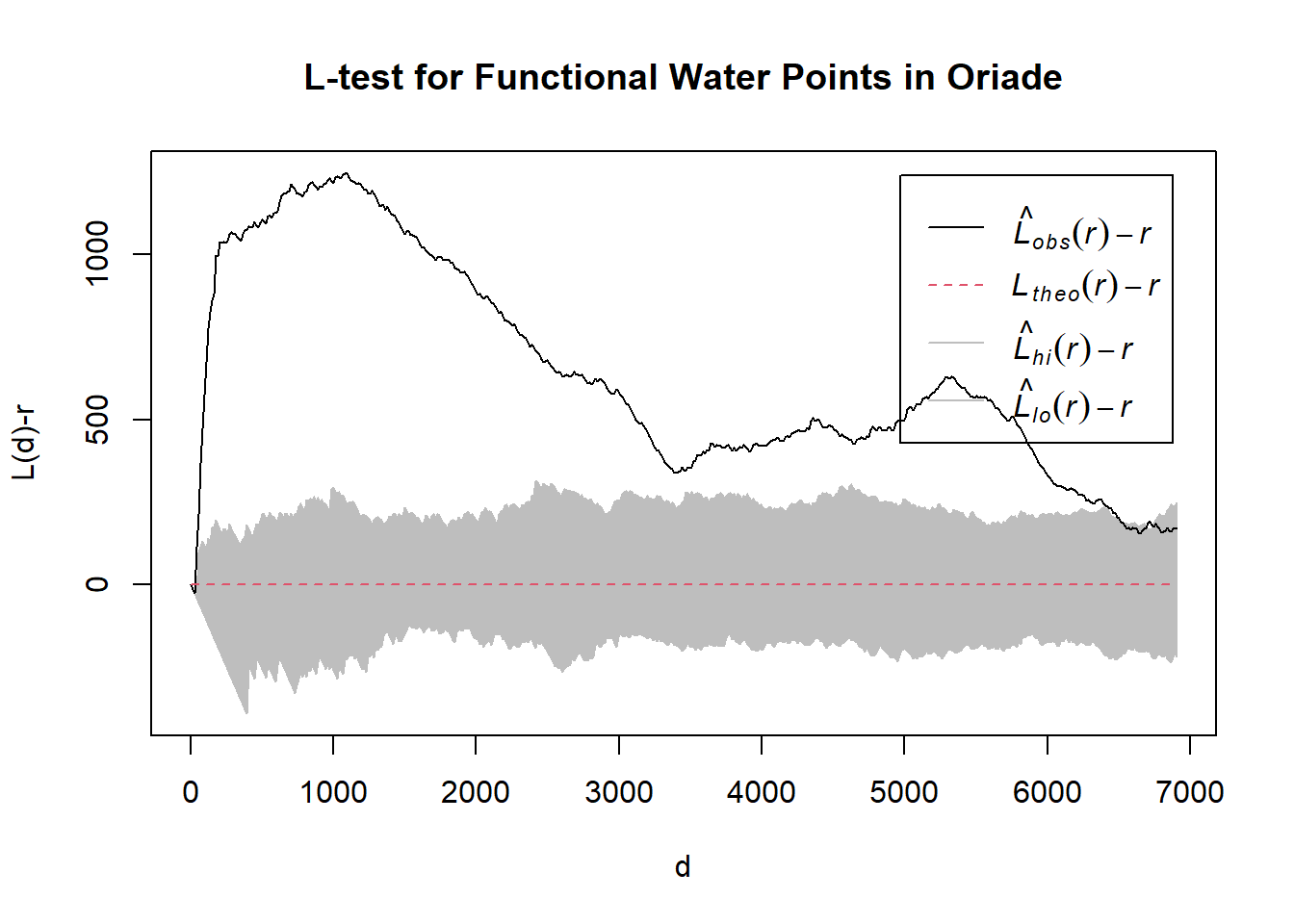
[1] "—————————————————————————————————————————————————————————————————————"
[1] "Test 29"
[1] "Now analyzing Administrative Level-2: Orolu"
Generating 39 simulations of CSR  ...
1, 2, 3, 4, 5, 6, 7, 8, 9, 10, 11, 12, 13, 14, 15, 16, 17, 18, 19, 20, 21, 22, 23, 24, 25, 26, 27, 28, 29, 30, 31, 32, 33, 34, 35, 36, 37, 38,  39.

Done.
[1] "—————————————————————————————————————————————————————————————————————"
[1] "Test 30"
[1] "Now analyzing Administrative Level-2: Osogbo"
Generating 39 simulations of CSR  ...
1, 2, 3, 4, 5, 6, 7, 8, 9, 10, 11, 12, 13, 14, 15, 16, 17, 18, 19, 20, 21, 22, 23, 24, 25, 26, 27, 28, 29, 30, 31, 32, 33, 34, 35, 36, 37, 38,  39.

Done.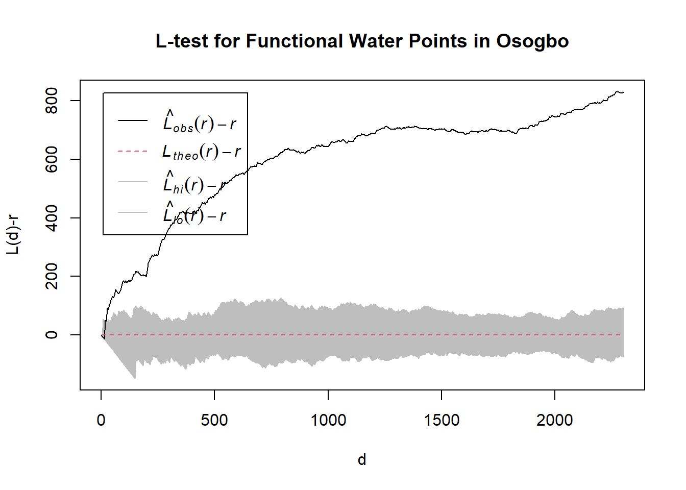
[1] "—————————————————————————————————————————————————————————————————————"for (i in 1:30){
print(paste("Now analyzing Administrative Level-2:", nga$ADM2_EN[i]))
nga1 = nga[i,]
nga_spat = as_Spatial(nga1)
nga_sp = as(nga_spat, "SpatialPolygons")
nga_owin = as(nga_sp, "owin")
wp_nonfunctional_R = wp_nonfunctional_ppp[nga_owin]
L_wp2.csr <- envelope(wp_nonfunctional_R, Lest, nsim = 39, rank = 1, glocal=TRUE)
title = paste("L-test for Non-Functional Water Points in", nga$ADM2_EN[i])
plot(L_wp2.csr, . - r ~ r, xlab="d", ylab="L(d)-r", main = title)
print("—————————————————————————————————————————————————————————————————————")
}[1] "Now analyzing Administrative Level-2: Aiyedade"
Generating 39 simulations of CSR ...
1, 2, 3, 4, 5, 6, 7, 8, 9, 10, 11, 12, 13, 14, 15, 16, 17, 18, 19, 20, 21, 22, 23, 24, 25, 26, 27, 28, 29, 30, 31, 32, 33, 34, 35, 36, 37, 38, 39.
Done.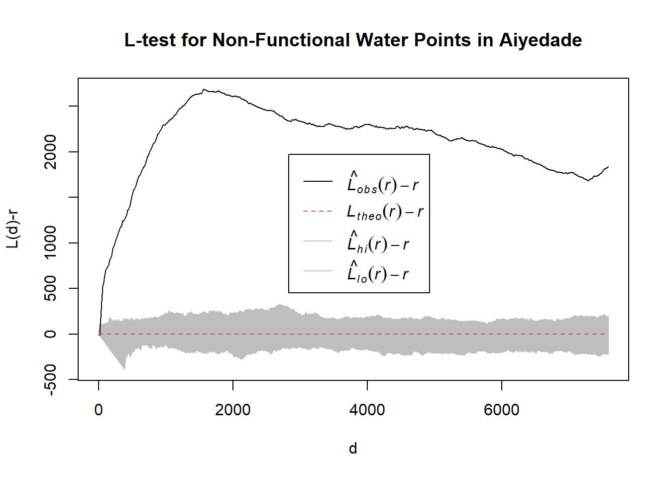
[1] "—————————————————————————————————————————————————————————————————————"
[1] "Now analyzing Administrative Level-2: Aiyedire"
Generating 39 simulations of CSR  ...
1, 2, 3, 4, 5, 6, 7, 8, 9, 10, 11, 12, 13, 14, 15, 16, 17, 18, 19, 20, 21, 22, 23, 24, 25, 26, 27, 28, 29, 30, 31, 32, 33, 34, 35, 36, 37, 38,  39.

Done.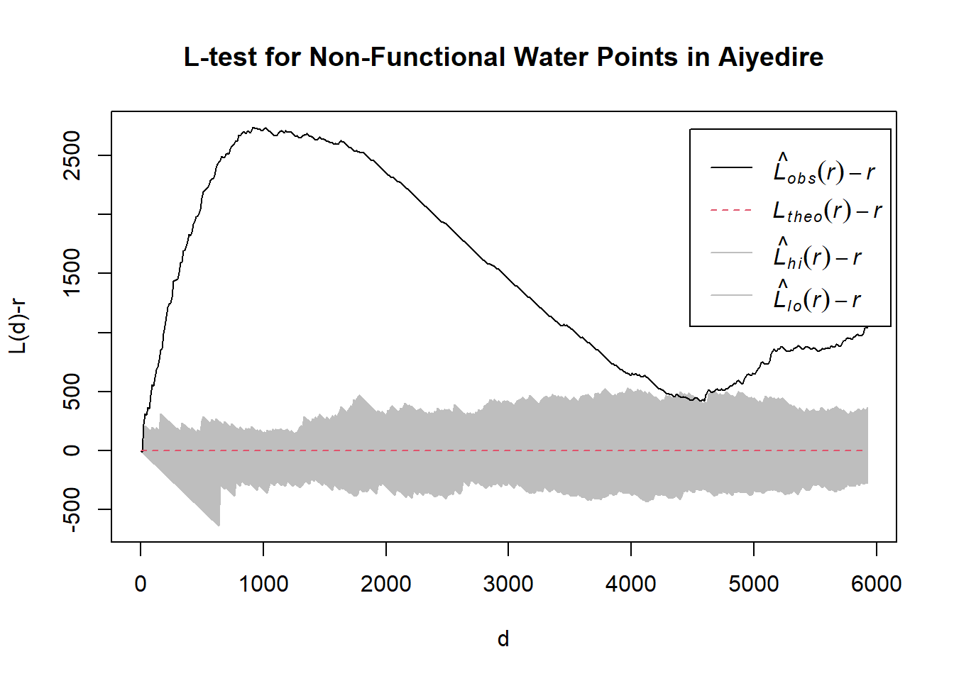
[1] "—————————————————————————————————————————————————————————————————————"
[1] "Now analyzing Administrative Level-2: Atakumosa East"
Generating 39 simulations of CSR  ...
1, 2, 3, 4, 5, 6, 7, 8, 9, 10, 11, 12, 13, 14, 15, 16, 17, 18, 19, 20, 21, 22, 23, 24, 25, 26, 27, 28, 29, 30, 31, 32, 33, 34, 35, 36, 37, 38,  39.

Done.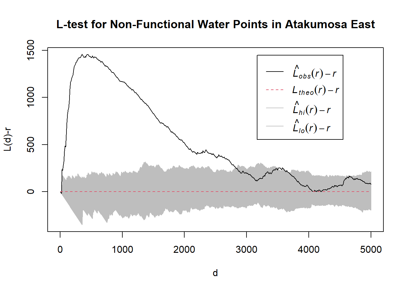
[1] "—————————————————————————————————————————————————————————————————————"
[1] "Now analyzing Administrative Level-2: Atakumosa West"
Generating 39 simulations of CSR  ...
1, 2, 3, 4, 5, 6, 7, 8, 9, 10, 11, 12, 13, 14, 15, 16, 17, 18, 19, 20, 21, 22, 23, 24, 25, 26, 27, 28, 29, 30, 31, 32, 33, 34, 35, 36, 37, 38,  39.

Done.
[1] "—————————————————————————————————————————————————————————————————————"
[1] "Now analyzing Administrative Level-2: Boluwaduro"
Generating 39 simulations of CSR  ...
1, 2, 3, 4, 5, 6, 7, 8, 9, 10, 11, 12, 13, 14, 15, 16, 17, 18, 19, 20, 21, 22, 23, 24, 25, 26, 27, 28, 29, 30, 31, 32, 33, 34, 35, 36, 37, 38,  39.

Done.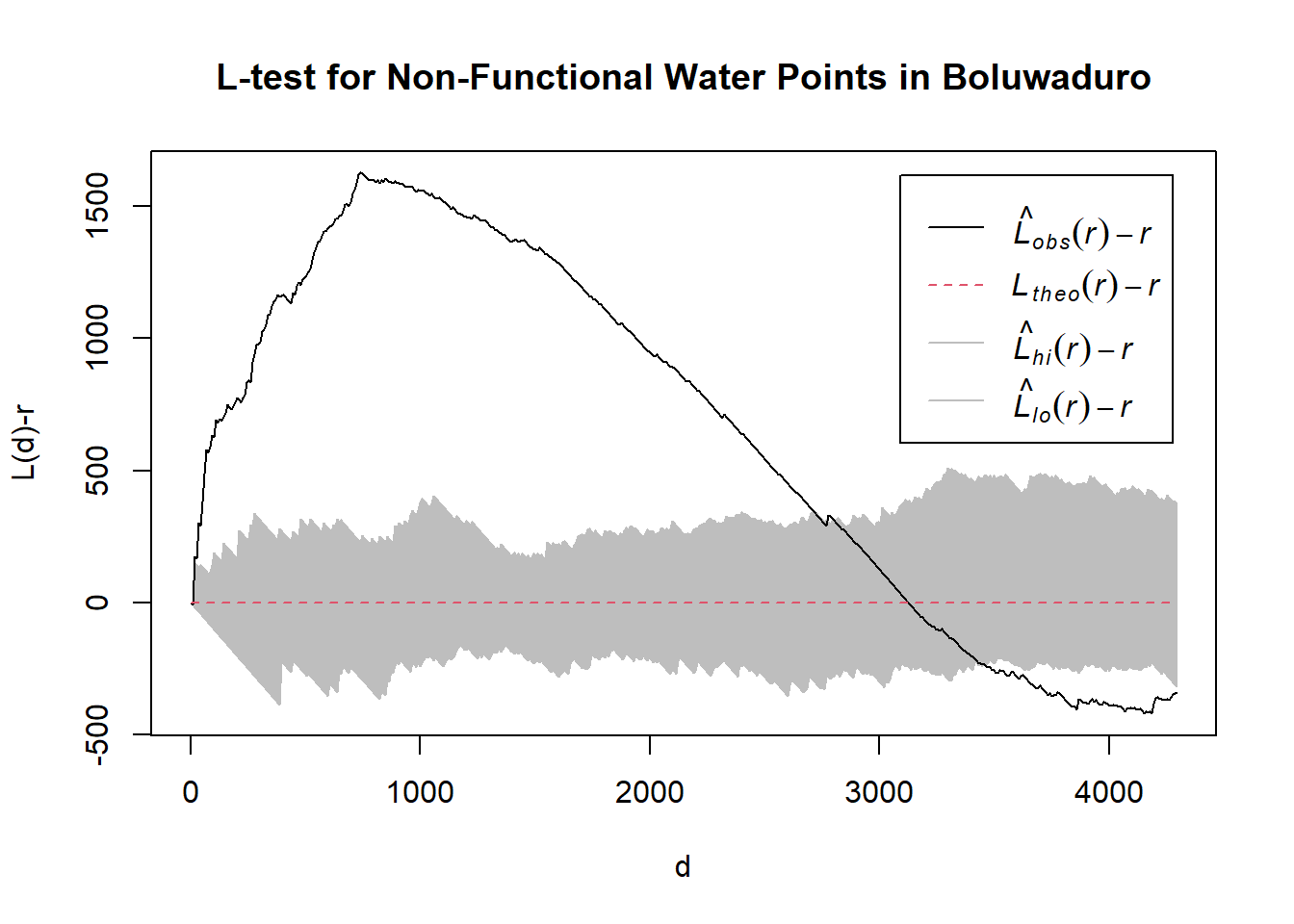
[1] "—————————————————————————————————————————————————————————————————————"
[1] "Now analyzing Administrative Level-2: Boripe"
Generating 39 simulations of CSR  ...
1, 2, 3, 4, 5, 6, 7, 8, 9, 10, 11, 12, 13, 14, 15, 16, 17, 18, 19, 20, 21, 22, 23, 24, 25, 26, 27, 28, 29, 30, 31, 32, 33, 34, 35, 36, 37, 38,  39.

Done.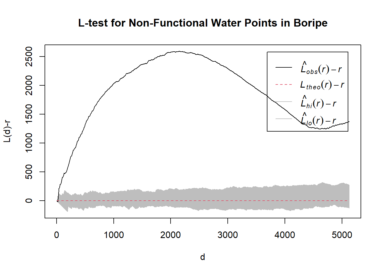
[1] "—————————————————————————————————————————————————————————————————————"
[1] "Now analyzing Administrative Level-2: Ede North"
Generating 39 simulations of CSR  ...
1, 2, 3, 4, 5, 6, 7, 8, 9, 10, 11, 12, 13, 14, 15, 16, 17, 18, 19, 20, 21, 22, 23, 24, 25, 26, 27, 28, 29, 30, 31, 32, 33, 34, 35, 36, 37, 38,  39.

Done.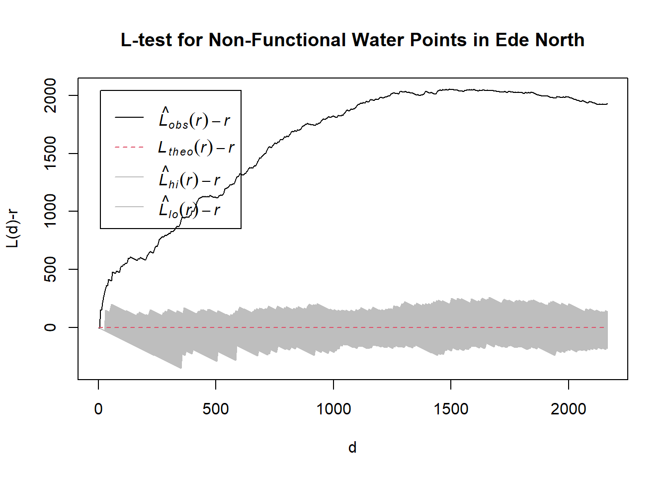
[1] "—————————————————————————————————————————————————————————————————————"
[1] "Now analyzing Administrative Level-2: Ede South"
Generating 39 simulations of CSR  ...
1, 2, 3, 4, 5, 6, 7, 8, 9, 10, 11, 12, 13, 14, 15, 16, 17, 18, 19, 20, 21, 22, 23, 24, 25, 26, 27, 28, 29, 30, 31, 32, 33, 34, 35, 36, 37, 38,  39.

Done.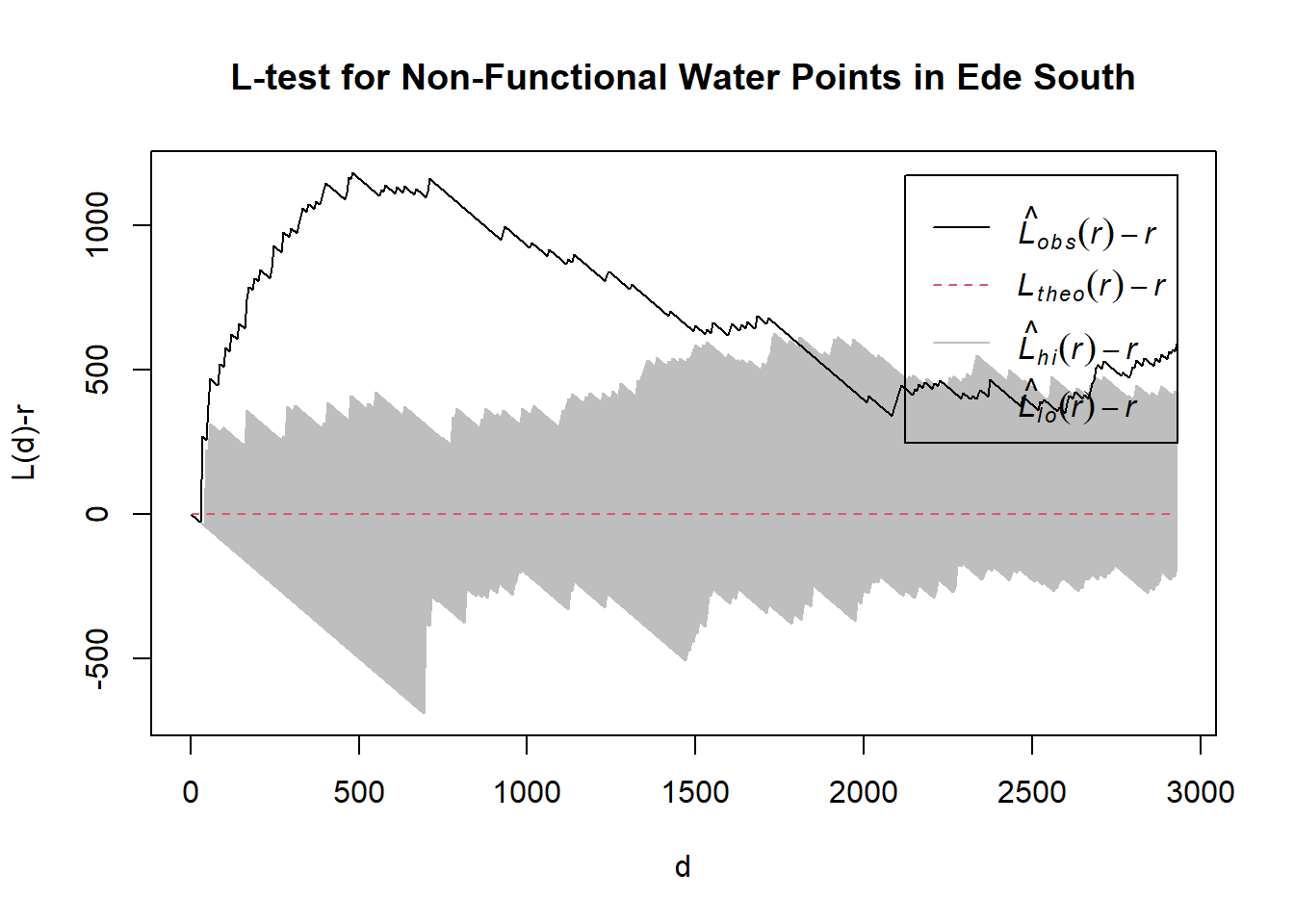
[1] "—————————————————————————————————————————————————————————————————————"
[1] "Now analyzing Administrative Level-2: Egbedore"
Generating 39 simulations of CSR  ...
1, 2, 3, 4, 5, 6, 7, 8, 9, 10, 11, 12, 13, 14, 15, 16, 17, 18, 19, 20, 21, 22, 23, 24, 25, 26, 27, 28, 29, 30, 31, 32, 33, 34, 35, 36, 37, 38,  39.

Done.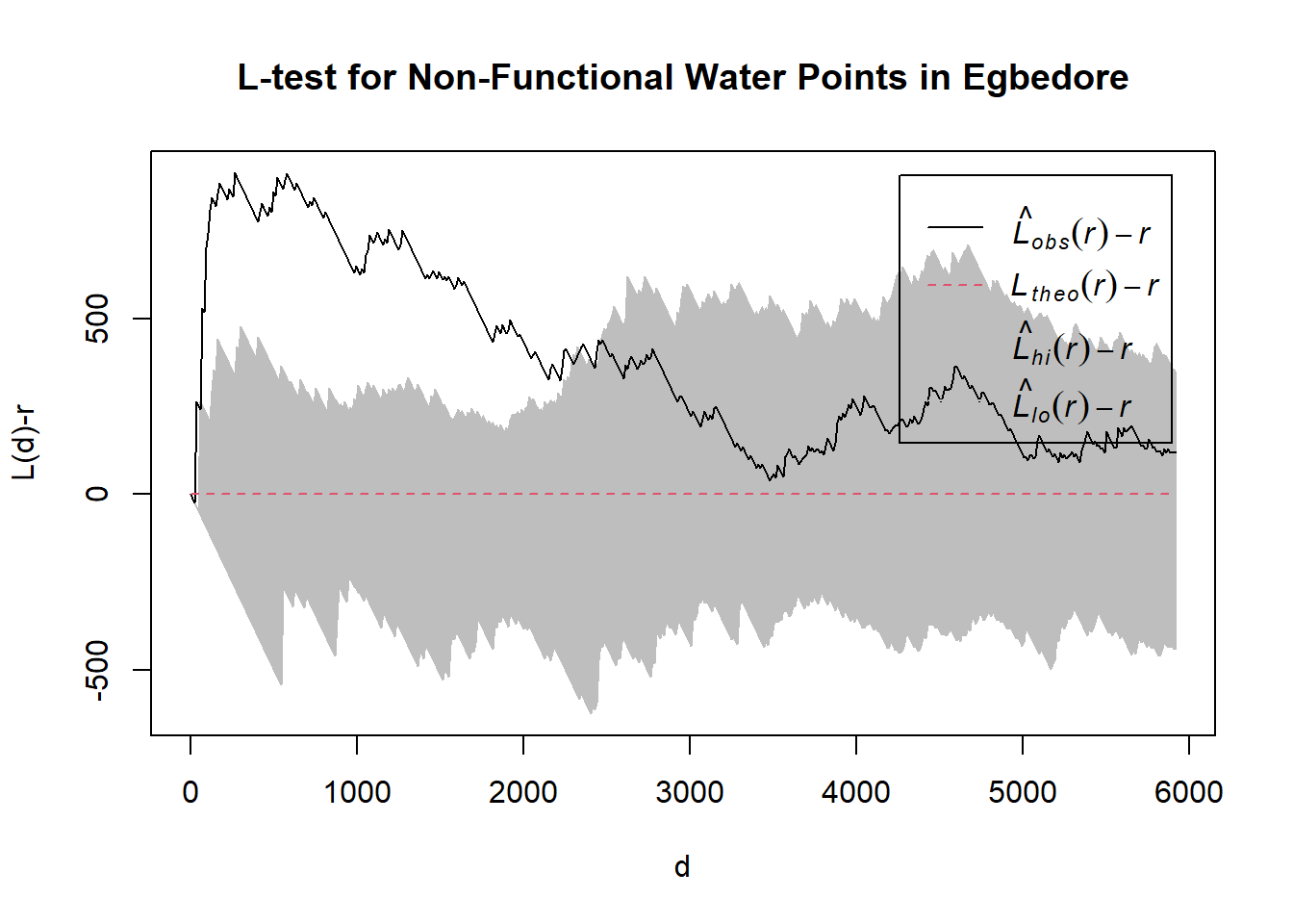
[1] "—————————————————————————————————————————————————————————————————————"
[1] "Now analyzing Administrative Level-2: Ejigbo"
Generating 39 simulations of CSR  ...
1, 2, 3, 4, 5, 6, 7, 8, 9, 10, 11, 12, 13, 14, 15, 16, 17, 18, 19, 20, 21, 22, 23, 24, 25, 26, 27, 28, 29, 30, 31, 32, 33, 34, 35, 36, 37, 38,  39.

Done.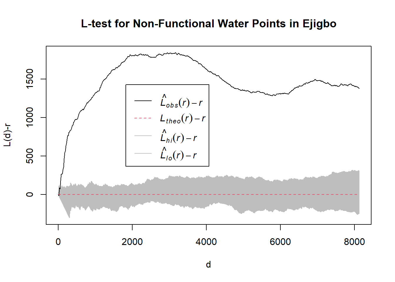
[1] "—————————————————————————————————————————————————————————————————————"
[1] "Now analyzing Administrative Level-2: Ife Central"
Generating 39 simulations of CSR  ...
1, 2, 3, 4, 5, 6, 7, 8, 9, 10, 11, 12, 13, 14, 15, 16, 17, 18, 19, 20, 21, 22, 23, 24, 25, 26, 27, 28, 29, 30, 31, 32, 33, 34, 35, 36, 37, 38,  39.

Done.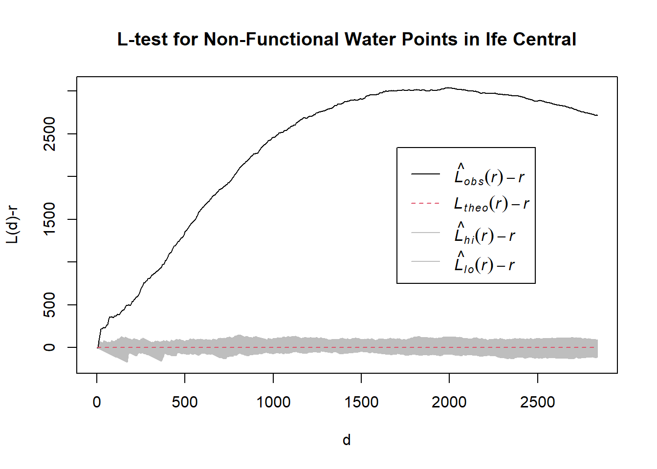
[1] "—————————————————————————————————————————————————————————————————————"
[1] "Now analyzing Administrative Level-2: Ife East"
Generating 39 simulations of CSR  ...
1, 2, 3, 4, 5, 6, 7, 8, 9, 10, 11, 12, 13, 14, 15, 16, 17, 18, 19, 20, 21, 22, 23, 24, 25, 26, 27, 28, 29, 30, 31, 32, 33, 34, 35, 36, 37, 38,  39.

Done.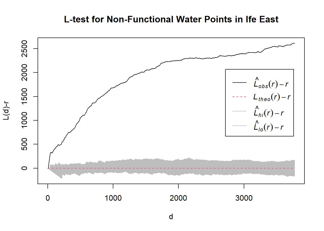
[1] "—————————————————————————————————————————————————————————————————————"
[1] "Now analyzing Administrative Level-2: Ife North"
Generating 39 simulations of CSR  ...
1, 2, 3, 4, 5, 6, 7, 8, 9, 10, 11, 12, 13, 14, 15, 16, 17, 18, 19, 20, 21, 22, 23, 24, 25, 26, 27, 28, 29, 30, 31, 32, 33, 34, 35, 36, 37, 38,  39.

Done.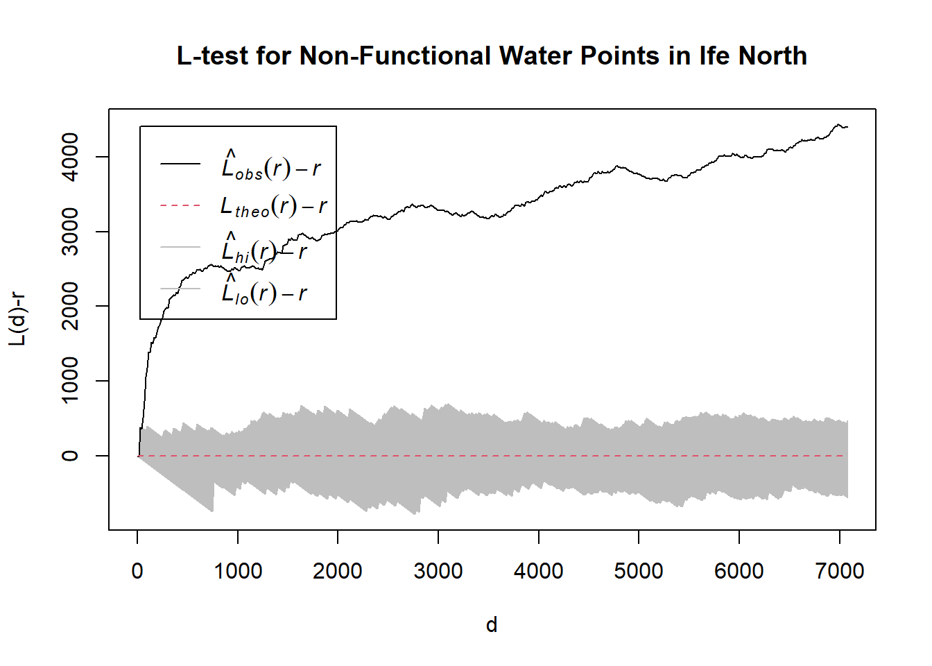
[1] "—————————————————————————————————————————————————————————————————————"
[1] "Now analyzing Administrative Level-2: Ife South"
Generating 39 simulations of CSR  ...
1, 2, 3, 4, 5, 6, 7, 8, 9, 10, 11, 12, 13, 14, 15, 16, 17, 18, 19, 20, 21, 22, 23, 24, 25, 26, 27, 28, 29, 30, 31, 32, 33, 34, 35, 36, 37, 38,  39.

Done.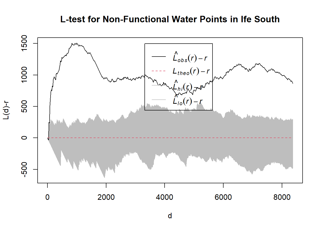
[1] "—————————————————————————————————————————————————————————————————————"
[1] "Now analyzing Administrative Level-2: Ifedayo"
Generating 39 simulations of CSR  ...
1, 2, 3, 4, 5, 6, 7, 8, 9, 10, 11, 12, 13, 14, 15, 16, 17, 18, 19, 20, 21, 22, 23, 24, 25, 26, 27, 28, 29, 30, 31, 32, 33, 34, 35, 36, 37, 38,  39.

Done.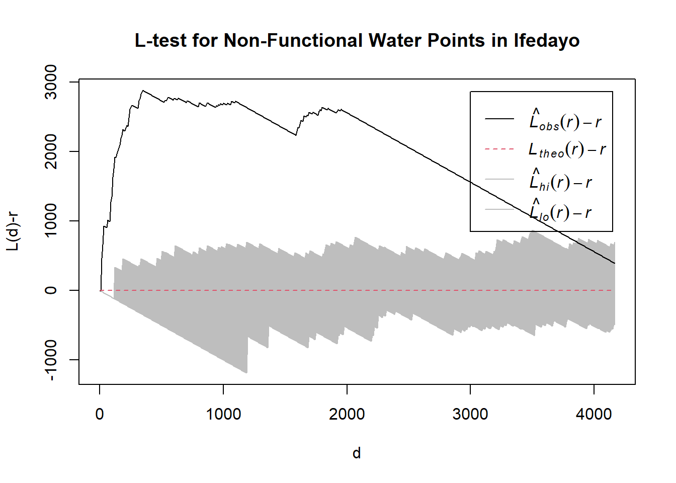
[1] "—————————————————————————————————————————————————————————————————————"
[1] "Now analyzing Administrative Level-2: Ifelodun"
Generating 39 simulations of CSR  ...
1, 2, 3, 4, 5, 6, 7, 8, 9, 10, 11, 12, 13, 14, 15, 16, 17, 18, 19, 20, 21, 22, 23, 24, 25, 26, 27, 28, 29, 30, 31, 32, 33, 34, 35, 36, 37, 38,  39.

Done.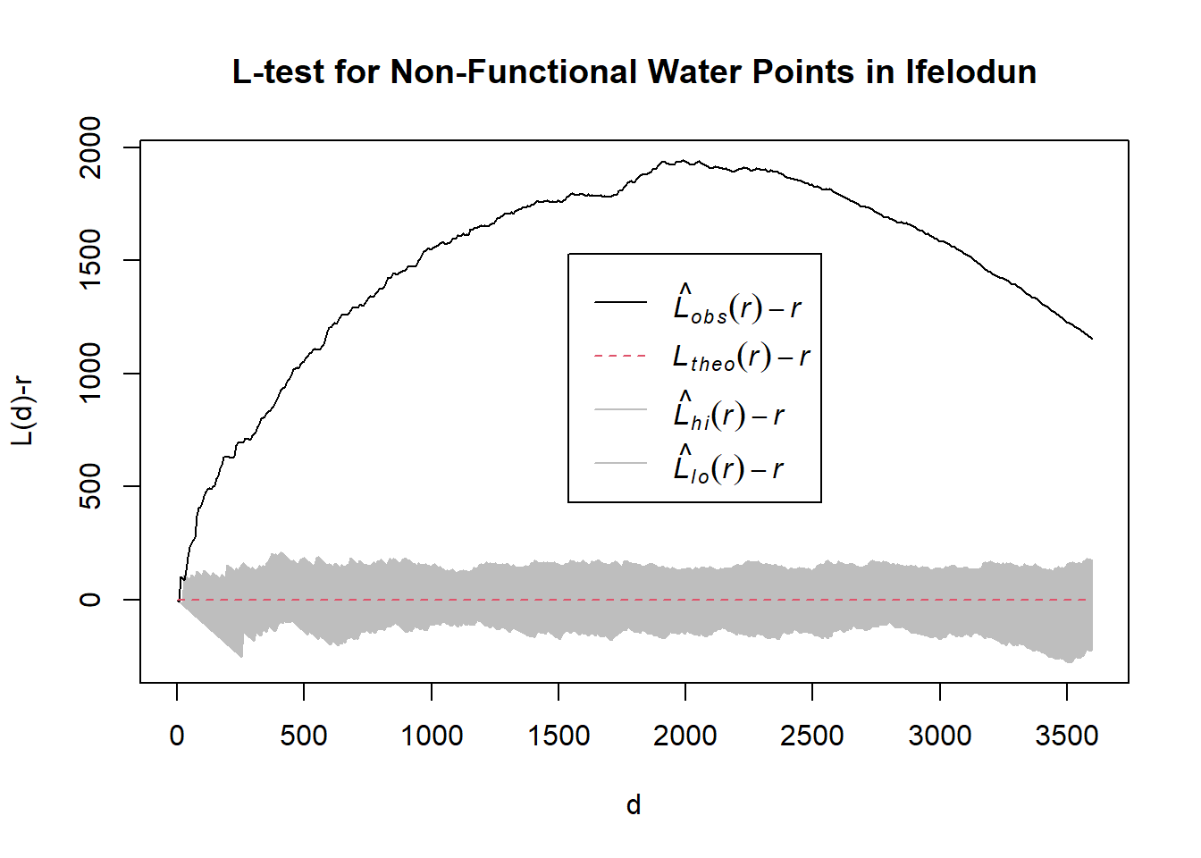
[1] "—————————————————————————————————————————————————————————————————————"
[1] "Now analyzing Administrative Level-2: Ila"
Generating 39 simulations of CSR  ...
1, 2, 3, 4, 5, 6, 7, 8, 9, 10, 11, 12, 13, 14, 15, 16, 17, 18, 19, 20, 21, 22, 23, 24, 25, 26, 27, 28, 29, 30, 31, 32, 33, 34, 35, 36, 37, 38,  39.

Done.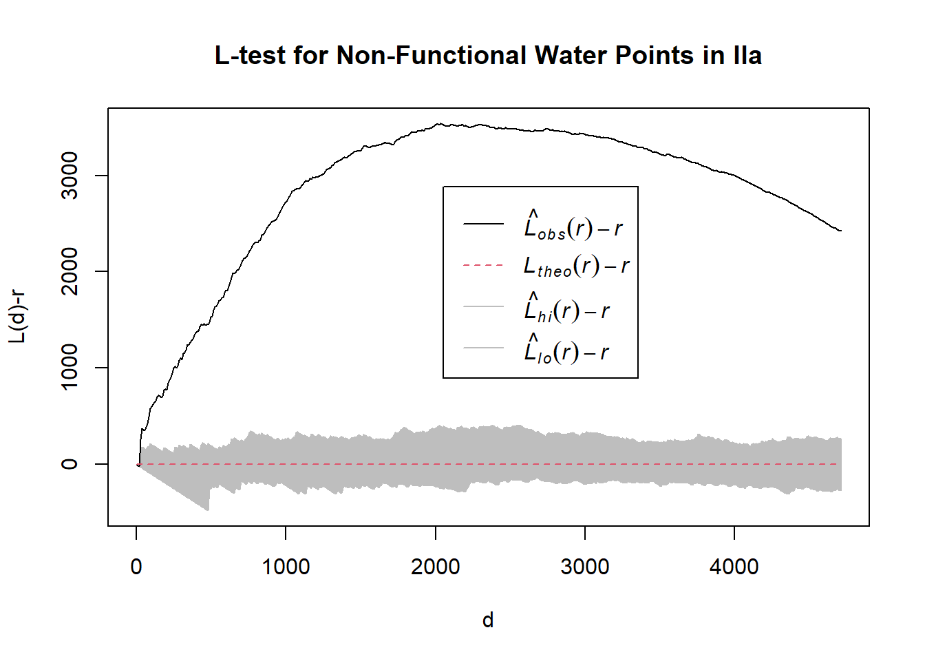
[1] "—————————————————————————————————————————————————————————————————————"
[1] "Now analyzing Administrative Level-2: Ilesha East"
Generating 39 simulations of CSR  ...
1, 2, 3, 4, 5, 6, 7, 8, 9, 10, 11, 12, 13, 14, 15, 16, 17, 18, 19, 20, 21, 22, 23, 24, 25, 26, 27, 28, 29, 30, 31, 32, 33, 34, 35, 36, 37, 38,  39.

Done.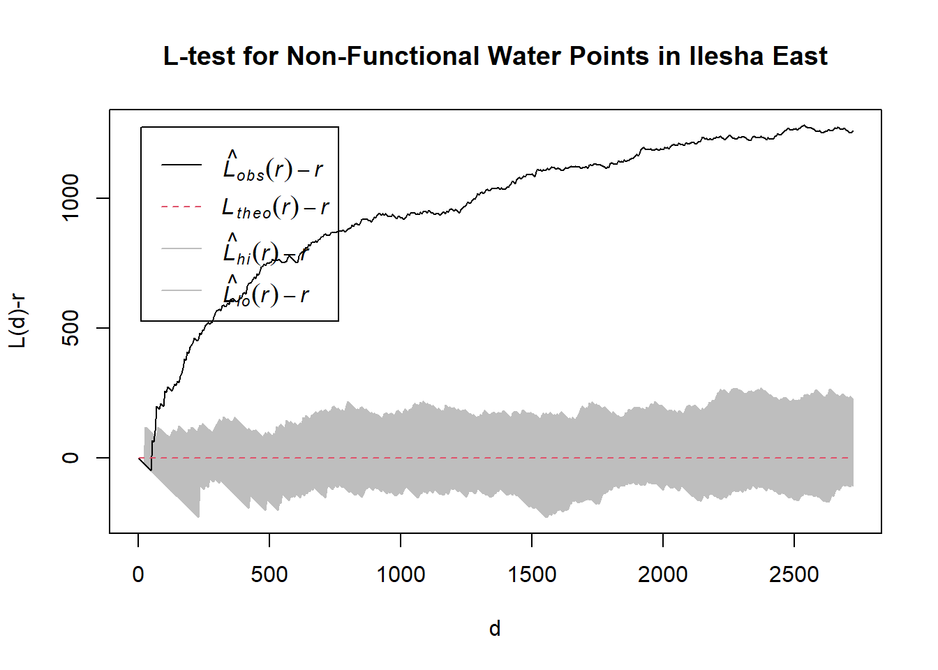
[1] "—————————————————————————————————————————————————————————————————————"
[1] "Now analyzing Administrative Level-2: Ilesha West"
Generating 39 simulations of CSR  ...
1, 2, 3, 4, 5, 6, 7, 8, 9, 10, 11, 12, 13, 14, 15, 16, 17, 18, 19, 20, 21, 22, 23, 24, 25, 26, 27, 28, 29, 30, 31, 32, 33, 34, 35, 36, 37, 38,  39.

Done.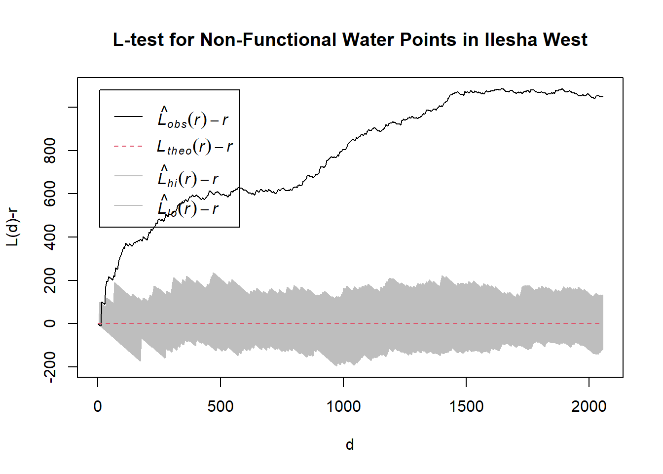
[1] "—————————————————————————————————————————————————————————————————————"
[1] "Now analyzing Administrative Level-2: Irepodun"
Generating 39 simulations of CSR  ...
1, 2, 3, 4, 5, 6, 7, 8, 9, 10, 11, 12, 13, 14, 15, 16, 17, 18, 19, 20, 21, 22, 23, 24, 25, 26, 27, 28, 29, 30, 31, 32, 33, 34, 35, 36, 37, 38,  39.

Done.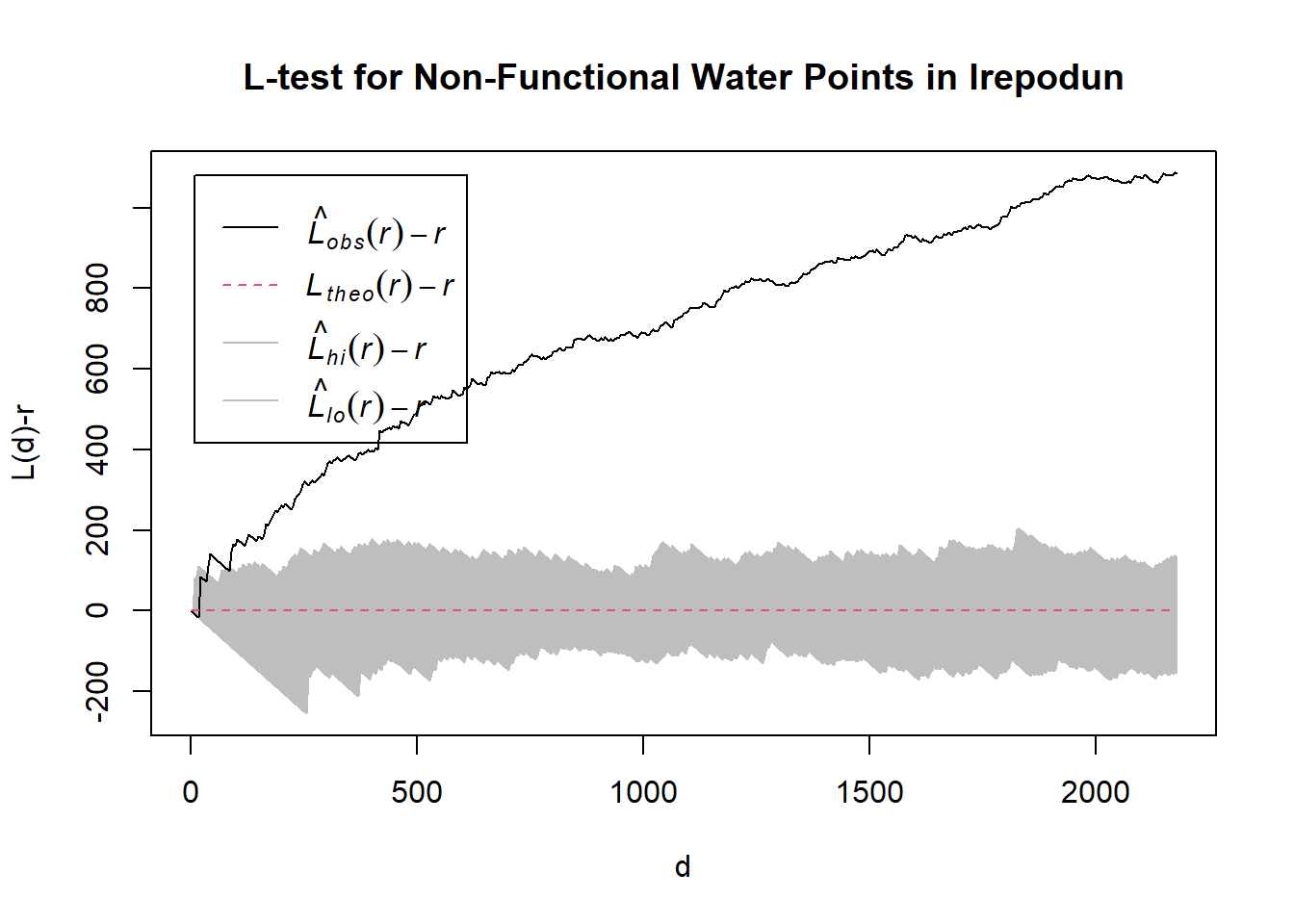
[1] "—————————————————————————————————————————————————————————————————————"
[1] "Now analyzing Administrative Level-2: Irewole"
Generating 39 simulations of CSR  ...
1, 2, 3, 4, 5, 6, 7, 8, 9, 10, 11, 12, 13, 14, 15, 16, 17, 18, 19, 20, 21, 22, 23, 24, 25, 26, 27, 28, 29, 30, 31, 32, 33, 34, 35, 36, 37, 38,  39.

Done.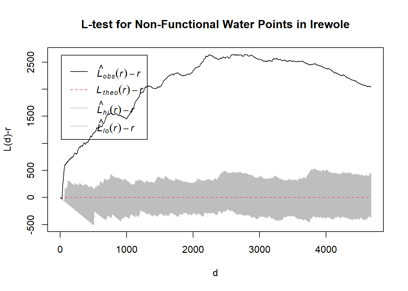
[1] "—————————————————————————————————————————————————————————————————————"
[1] "Now analyzing Administrative Level-2: Isokan"
Generating 39 simulations of CSR  ...
1, 2, 3, 4, 5, 6, 7, 8, 9, 10, 11, 12, 13, 14, 15, 16, 17, 18, 19, 20, 21, 22, 23, 24, 25, 26, 27, 28, 29, 30, 31, 32, 33, 34, 35, 36, 37, 38,  39.

Done.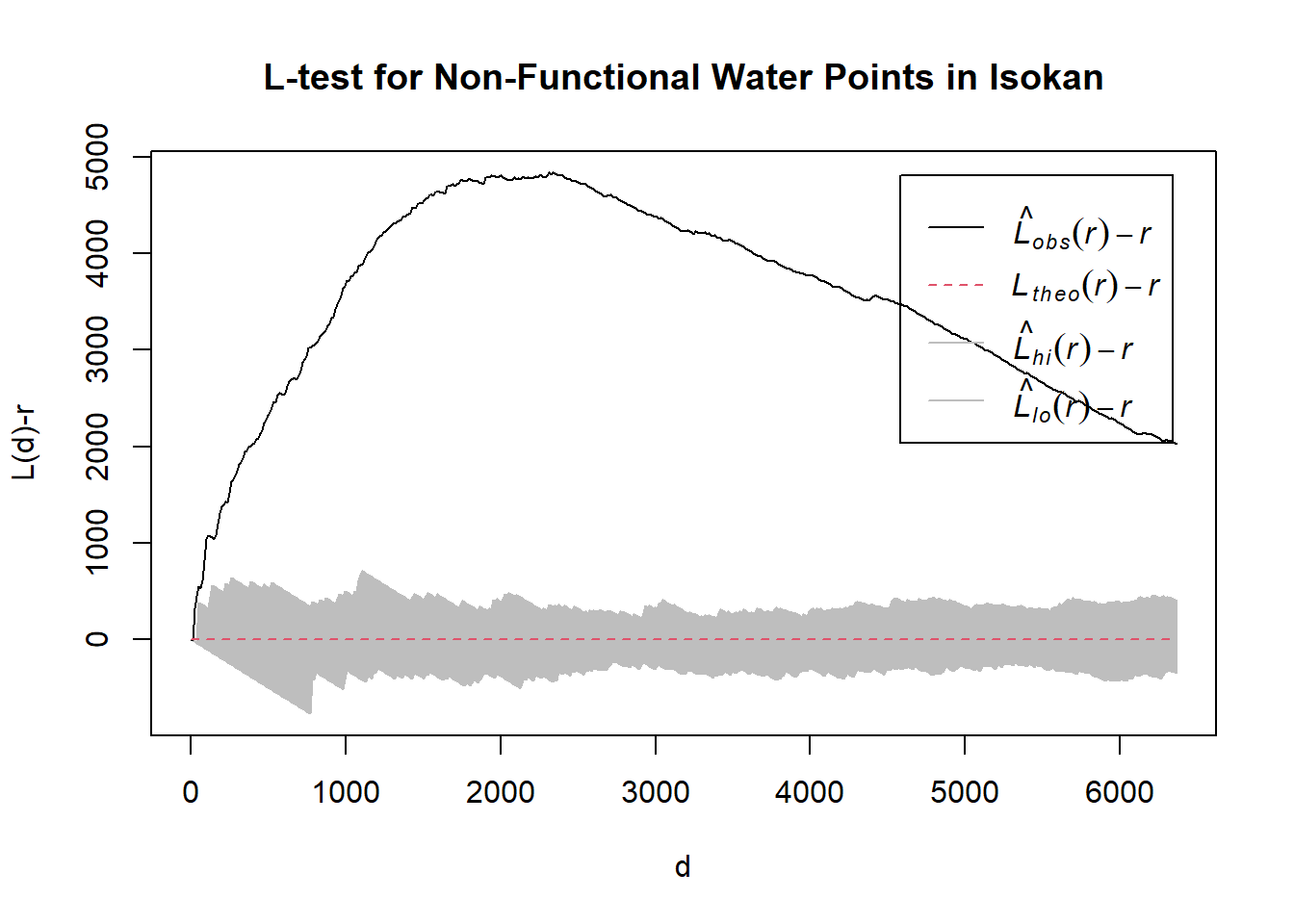
[1] "—————————————————————————————————————————————————————————————————————"
[1] "Now analyzing Administrative Level-2: Iwo"
Generating 39 simulations of CSR  ...
1, 2, 3, 4, 5, 6, 7, 8, 9, 10, 11, 12, 13, 14, 15, 16, 17, 18, 19, 20, 21, 22, 23, 24, 25, 26, 27, 28, 29, 30, 31, 32, 33, 34, 35, 36, 37, 38,  39.

Done.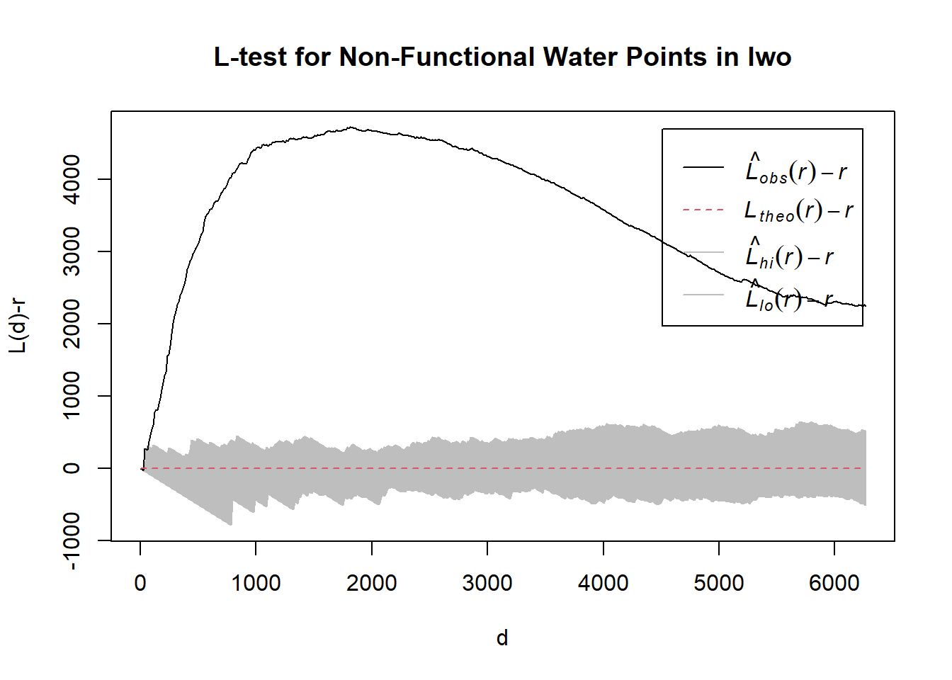
[1] "—————————————————————————————————————————————————————————————————————"
[1] "Now analyzing Administrative Level-2: Obokun"
Generating 39 simulations of CSR  ...
1, 2, 3, 4, 5, 6, 7, 8, 9, 10, 11, 12, 13, 14, 15, 16, 17, 18, 19, 20, 21, 22, 23, 24, 25, 26, 27, 28, 29, 30, 31, 32, 33, 34, 35, 36, 37, 38,  39.

Done.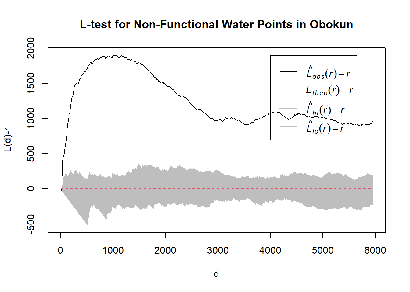
[1] "—————————————————————————————————————————————————————————————————————"
[1] "Now analyzing Administrative Level-2: Odo-Otin"
Generating 39 simulations of CSR  ...
1, 2, 3, 4, 5, 6, 7, 8, 9, 10, 11, 12, 13, 14, 15, 16, 17, 18, 19, 20, 21, 22, 23, 24, 25, 26, 27, 28, 29, 30, 31, 32, 33, 34, 35, 36, 37, 38,  39.

Done.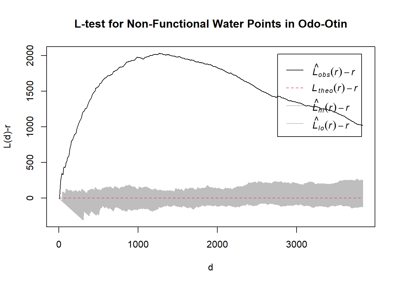
[1] "—————————————————————————————————————————————————————————————————————"
[1] "Now analyzing Administrative Level-2: Ola-oluwa"
Generating 39 simulations of CSR  ...
1, 2, 3, 4, 5, 6, 7, 8, 9, 10, 11, 12, 13, 14, 15, 16, 17, 18, 19, 20, 21, 22, 23, 24, 25, 26, 27, 28, 29, 30, 31, 32, 33, 34, 35, 36, 37, 38,  39.

Done.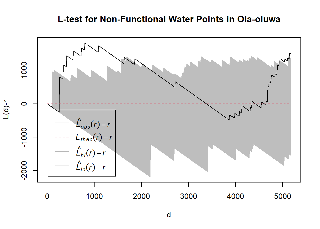
[1] "—————————————————————————————————————————————————————————————————————"
[1] "Now analyzing Administrative Level-2: Olorunda"
Generating 39 simulations of CSR  ...
1, 2, 3, 4, 5, 6, 7, 8, 9, 10, 11, 12, 13, 14, 15, 16, 17, 18, 19, 20, 21, 22, 23, 24, 25, 26, 27, 28, 29, 30, 31, 32, 33, 34, 35, 36, 37, 38,  39.

Done.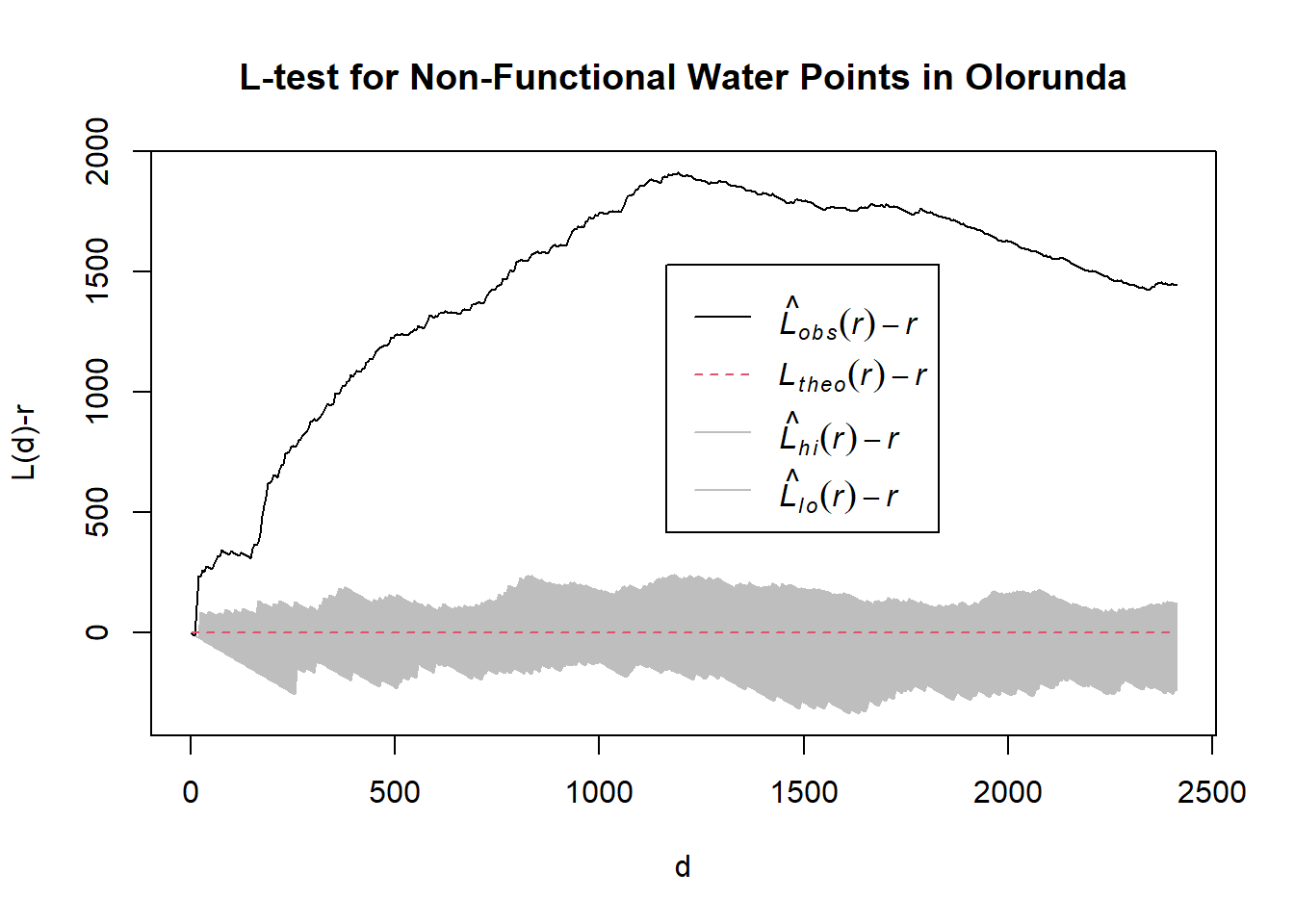
[1] "—————————————————————————————————————————————————————————————————————"
[1] "Now analyzing Administrative Level-2: Oriade"
Generating 39 simulations of CSR  ...
1, 2, 3, 4, 5, 6, 7, 8, 9, 10, 11, 12, 13, 14, 15, 16, 17, 18, 19, 20, 21, 22, 23, 24, 25, 26, 27, 28, 29, 30, 31, 32, 33, 34, 35, 36, 37, 38,  39.

Done.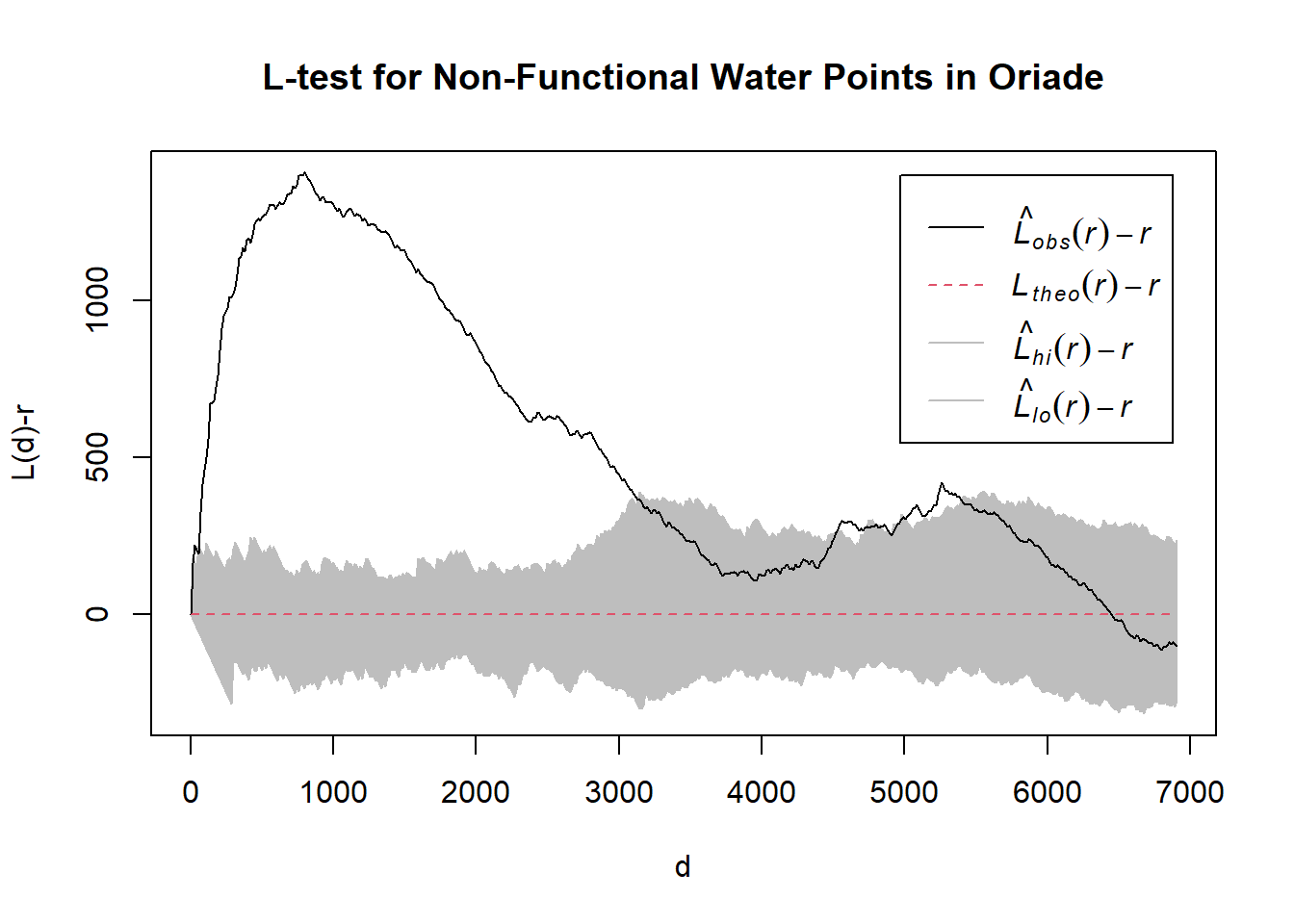
[1] "—————————————————————————————————————————————————————————————————————"
[1] "Now analyzing Administrative Level-2: Orolu"
Generating 39 simulations of CSR  ...
1, 2, 3, 4, 5, 6, 7, 8, 9, 10, 11, 12, 13, 14, 15, 16, 17, 18, 19, 20, 21, 22, 23, 24, 25, 26, 27, 28, 29, 30, 31, 32, 33, 34, 35, 36, 37, 38,  39.

Done.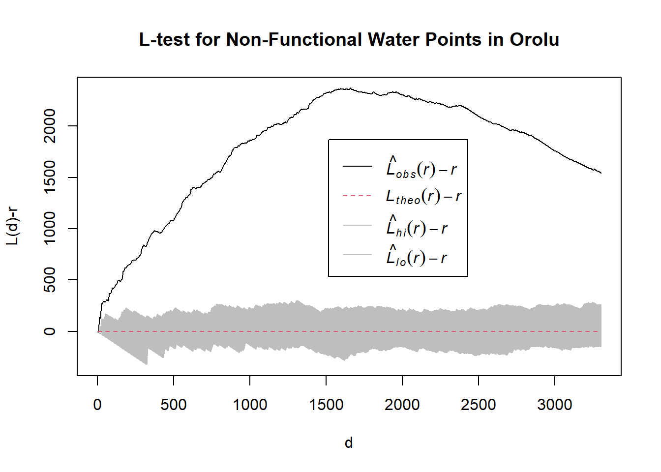
[1] "—————————————————————————————————————————————————————————————————————"
[1] "Now analyzing Administrative Level-2: Osogbo"
Generating 39 simulations of CSR  ...
1, 2, 3, 4, 5, 6, 7, 8, 9, 10, 11, 12, 13, 14, 15, 16, 17, 18, 19, 20, 21, 22, 23, 24, 25, 26, 27, 28, 29, 30, 31, 32, 33, 34, 35, 36, 37, 38,  39.

Done.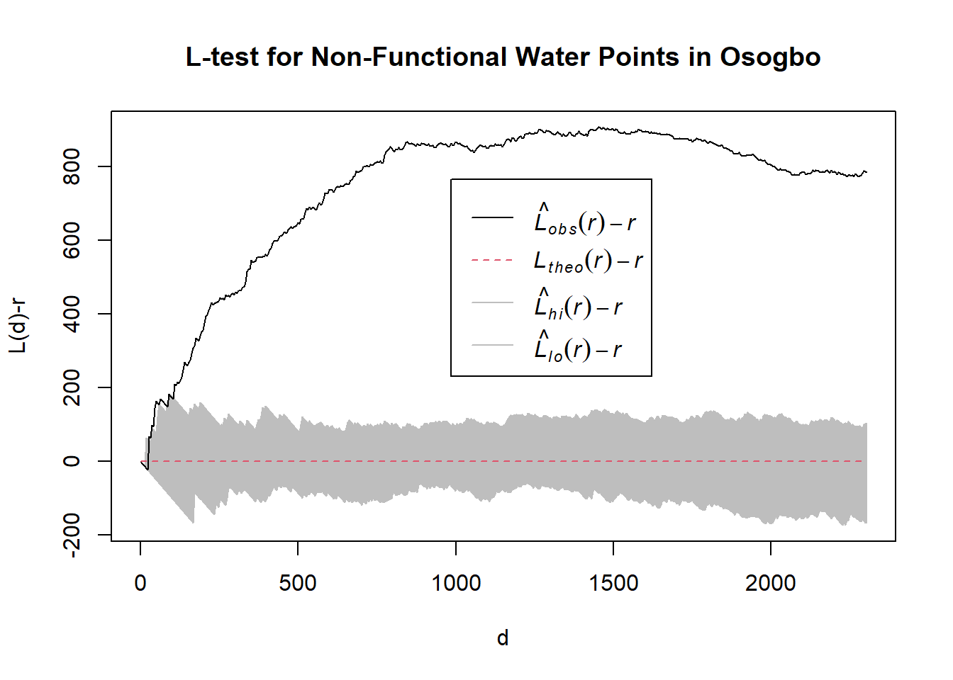
[1] "—————————————————————————————————————————————————————————————————————"To make the purpose of drawing statistical conclusion, I will walk you through the interpretation of the first three level-2 administrative boundaries for functional water points.
Looking at the Aiyedade boundary, we see that the observed L value is above the theoretical line and directly jumps above the envelope. Given our observation, we can conclude that at a 5% significance level, the functional water points in Aiyedade are concentrated. Spatial clustering is statistically significant.
Looking at the Aiyedire boundary, we have the same statistical conclusion. The L values are always above the upper limit of the envelope, meaning that spatial clustering of functional water points is statistically significant at a 5% signifance level.
Finally, looking at the Atakumose East boundary, we see that at a distance of 0 to 2100, L values are above the higher limit of the envelope, so the clustering is statistically significant. Between distances of 2100 - 3900 and 4100 - 5000, the L values are located within the envelope, so spatial clustering for these distances is not significant. Between distances of 3900 and 4100, the L values are below the lower limit of the envelope, meaning that spatial dispersion for these distances is statistically significant.
In this section, you are required to confirm statistically if the spatial distribution of functional and non-functional water points are independent from each other.
First, we rename the status into two main groups, functional and non-functional. It will help us in our local collocation quotient analysis. Using the mutate() and recode() functions, we can do as explained above.
water_points = wp_sf_nga %>%
  mutate(status_clean = recode(status_clean, "Functional but not in use" = 'Functional', "Functional but needs repair" = 'Functional', "Abandoned/Decommissioned" = 'Non-Functional', "Abandoned" = 'Non-Functional', "Non-Functional due to dry season" = 'Non-Functional')) %>%
  filter(status_clean %in%
           c("Functional",
             "Non-Functional"))
We then visualize the new categories on a map using the tmap package.
tmap_mode("view")
tm_shape(nga)+
  tm_polygons()+
tm_shape(st_intersection(water_points, nga))+
  tm_dots(col = "status_clean",
          size = 0.01,
          border.col = "black",
          border.lwd = 0.5)+
tm_view(set.zoom.limits = c(9, 12))H0 : Functional and Non-Functional Water Points are randomly distributed
H1 : Functional and Non-Functional Water Points are not randomly distributed (e.g.,they are collocated or isolated)
We will use a 5% significance level, in other words, a 95% confidence level.
nb = include_self(st_knn(st_geometry(water_points), 6))

wt = st_kernel_weights(nb, water_points, "gaussian", adaptive = TRUE)
functional = water_points %>%
filter(status_clean %in%
c("Functional",
"Functional but not in use",
"Functional but needs repair"))
A = functional$status_cleannonfunctional = water_points %>%
filter(status_clean %in%
c("Abandoned/Decommissioned",
"Abandoned",
"Non-Functional due to dry season",
"Non-Functional"))
B = nonfunctional$status_cleanLCLQ = local_colocation(A, B, nb, wt, 99)LCLQ_wp = cbind(water_points, LCLQ)tmap_mode("view")
tm_shape(nga)+
tm_polygons()+
tm_shape(st_intersection(LCLQ_wp, nga))+
tm_dots(col = c("Non.Functional"),
size = 0.01,
border.col = "black",
border.lwd = 0.5)+
tm_view(set.zoom.limits = c(9, 12))tmap_mode("plot")head(LCLQ_wp[order(LCLQ_wp$p_sim_Non.Functional),])Simple feature collection with 6 features and 3 fields
Geometry type: POINT
Dimension: XY
Bounding box: xmin: 221679.6 ymin: 383929.1 xmax: 236412 ymax: 413752
Projected CRS: Minna / Nigeria West Belt
status_clean Non.Functional p_sim_Non.Functional Geometry
60 Functional 0.9995411 0.01 POINT (233001.2 391744.6)
115 Functional 0.9995411 0.01 POINT (223962.7 413164)
116 Functional 0.9995411 0.01 POINT (232691.4 413752)
119 Functional 0.9995411 0.01 POINT (221679.6 404712.7)
146 Functional 0.9995411 0.01 POINT (236412 383929.1)
260 Functional 0.9995411 0.01 POINT (223015.1 412900.8)When cross referencing the points indicated on our above map as statistically significant and our data frame, we observe that their Local Collocation Quotient tends towards 1. It means that for each feature A – namely Functional Water Points - it is as likely to have a category B feature – Non-Functional Water Points - as we might expect (interpretation based on ArcGIS Pro tool referencing).