In-Class Exercise -

Author

Pierre HAAS

Published

February 13, 2023

Modified

March 19, 2023

1 Getting Started

1.1 Installing and Loading Packages

pacman::p_load(sf, sfdep, tmap, tidyverse)

1.2 Import data sets

1.2.1 Aspatial data

hunan2012 = read_csv("data/aspatial/Hunan_2012.csv")
head(hunan2012)

# A tibble: 6 × 29
  County   City  avg_w…¹ depos…²   FAI Gov_Rev Gov_Exp    GDP GDPPC    GIO  Loan
  <chr>    <chr>   <dbl>   <dbl> <dbl>   <dbl>   <dbl>  <dbl> <dbl>  <dbl> <dbl>
1 Anhua    Yiya…   30544  10967  6832.    457.   2703  13225  14567  9277. 3955.
2 Anren    Chen…   28058   4599. 6386.    221.   1455.  4941. 12761  4189. 2555.
3 Anxiang  Chan…   31935   5517. 3541     244.   1780. 12482  23667  5109. 2807.
4 Baojing  Huna…   30843   2250  1005.    193.   1379.  4088. 14563  3624. 1254.
5 Chaling  Zhuz…   31251   8241. 6508.    620.   1947  11585  20078  9158. 4287.
6 Changni… Heng…   28518  10860  7920     770.   2632. 19886  24418 37392  4243.
# … with 18 more variables: NIPCR <dbl>, Bed <dbl>, Emp <dbl>, EmpR <dbl>,
#   EmpRT <dbl>, Pri_Stu <dbl>, Sec_Stu <dbl>, Household <dbl>,
#   Household_R <dbl>, NOIP <dbl>, Pop_R <dbl>, RSCG <dbl>, Pop_T <dbl>,
#   Agri <dbl>, Service <dbl>, Disp_Inc <dbl>, RORP <dbl>, ROREmp <dbl>, and
#   abbreviated variable names ¹avg_wage, ²deposite

1.2.2 Geospatial data

hunanGeo = st_read(dsn = "data/geospatial",
                   layer = "Hunan")

Reading layer `Hunan' from data source 
  `C:\p-haas\IS415\In-class_Ex\In-class_Ex06\data\geospatial' 
  using driver `ESRI Shapefile'
Simple feature collection with 88 features and 7 fields
Geometry type: POLYGON
Dimension:     XY
Bounding box:  xmin: 108.7831 ymin: 24.6342 xmax: 114.2544 ymax: 30.12812
Geodetic CRS:  WGS 84

glimpse(hunanGeo)

Rows: 88
Columns: 8
$ NAME_2     <chr> "Changde", "Changde", "Changde", "Changde", "Changde", "Cha…
$ ID_3       <int> 21098, 21100, 21101, 21102, 21103, 21104, 21109, 21110, 211…
$ NAME_3     <chr> "Anxiang", "Hanshou", "Jinshi", "Li", "Linli", "Shimen", "L…
$ ENGTYPE_3  <chr> "County", "County", "County City", "County", "County", "Cou…
$ Shape_Leng <dbl> 1.869074, 2.360691, 1.425620, 3.474325, 2.289506, 4.171918,…
$ Shape_Area <dbl> 0.10056190, 0.19978745, 0.05302413, 0.18908121, 0.11450357,…
$ County     <chr> "Anxiang", "Hanshou", "Jinshi", "Li", "Linli", "Shimen", "L…
$ geometry   <POLYGON [°]> POLYGON ((112.0625 29.75523..., POLYGON ((112.2288 …

1.3 Combining data frames

hunan_gdppc = left_join(hunanGeo, hunan2012) %>%
  select(1:4, 7, 15)

Note that we keep columns NAME_3 and County to double check that the left join was done correctly and that spelling is the same across the two columns.

1.4 Plotting a Choropleth map

tm_shape(hunan_gdppc)+
  tm_fill("GDPPC",
          style = "quantile",
          palette = "Blues",
          title = "GDP / cap")+
  tm_layout(main.title = "Distribution of GDP per capita by ",
          main.title.position = "center",
          main.title.size = 1.2,
          legend.height = 0.45,
          legend.width = 0.35,
          frame = TRUE)+
  tm_borders(alpha = 0.5)+
  tm_compass(type = "8star", size = 2)+
  tm_scale_bar()+
  tm_grid(alpha = 0.2)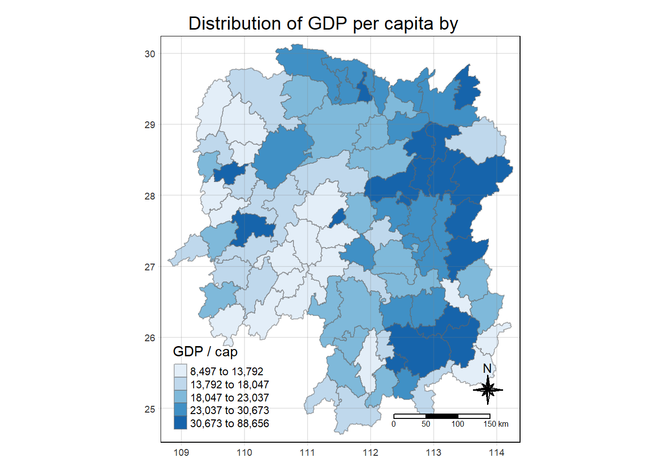

1.5 Contiguity Neighbors Analysis

Using the Queen method

cn_queen = hunan_gdppc %>%
  mutate(nb = st_contiguity(geometry),
         .before = 1)

Using the Rooks method

cn_rooks = hunan_gdppc %>%
  mutate(nb = st_contiguity(geometry, queen = FALSE),
         .before = 1)

1.6 Computing Contiguity Weights

Using the Queen method

wm_q = hunan_gdppc %>%
  mutate(nb = st_contiguity(geometry),
         wt = st_weights(nb),
         .before = 1)

Using the Rooks method

wm_r = hunan_gdppc %>%
  mutate(nb = st_contiguity(geometry),
         queen = FALSE,
         wt = st_weights(nb),
         .before = 1)